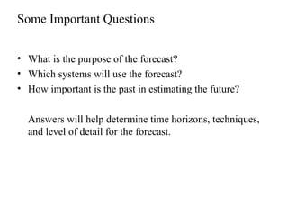
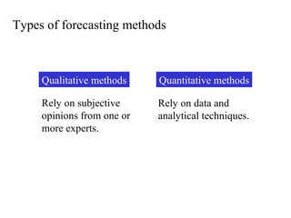
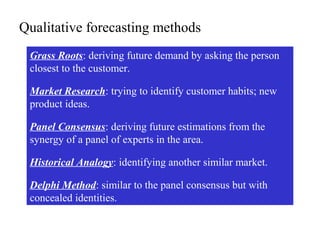
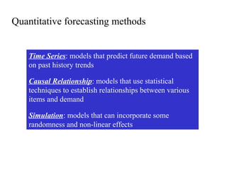
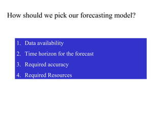
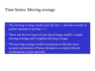
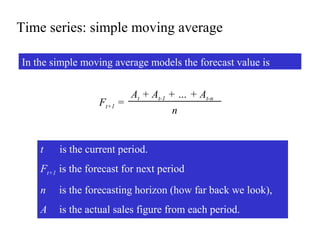
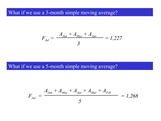
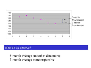
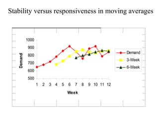
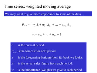
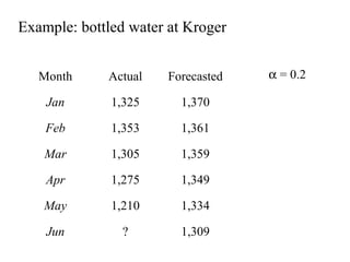
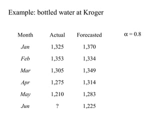
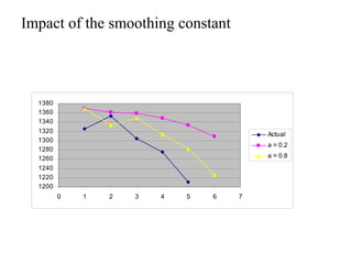
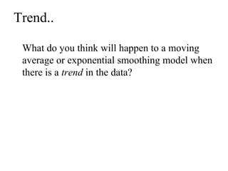
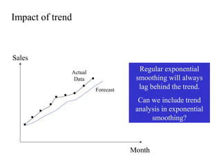
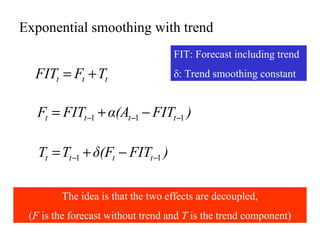
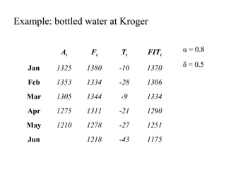
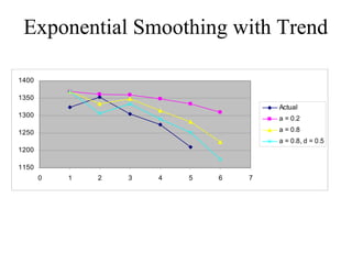
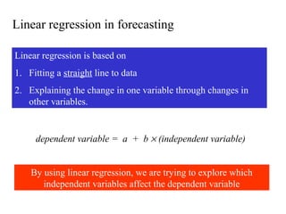
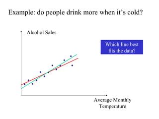
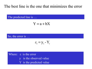
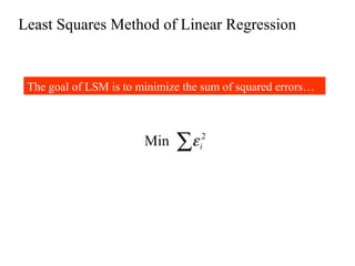
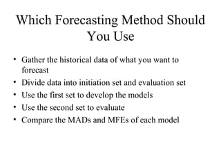
ForecastingForecasting
““Prediction is very difficult,Prediction is very difficult,
especially if it's about the future.especially if it's about the future.””
Nils BohrNils Bohr
Objectives
• Give the fundamental rules of forecasting
• Calculate a forecast using a moving average,
weighted moving average, and exponential
smoothing
• Calculate the accuracy of a forecast
What is forecasting?
Forecasting is a tool used for predicting
future demand based on
past demand information.
Why is forecasting important?
Demand for products and services is usually uncertain.
Forecasting can be used for…
• Strategic planning (long range planning)
• Finance and accounting (budgets and cost controls)
• Marketing (future sales, new products)
• Production and operations
What is forecasting all about?
Demand for Mercedes E Class
Time
Jan Feb Mar Apr May Jun Jul Aug
Actual demand (past sales)
Predicted demand
We try to predict the
future by looking back
at the past
Predicted
demand
looking
back six
months
From the March 10, 2006 WSJ:
Ahead of the Oscars, an economics professor, at the request of Weekend
Journal, processed data about this year's films nominated for best picture
through his statistical model and predicted with 97.4% certainty that
"Brokeback Mountain" would win. Oops. Last year, the professor tuned his
model until it correctly predicted 18 of the previous 20 best-picture awards;
then it predicted that "The Aviator" would win; "Million Dollar Baby" won
instead.
Sometimes models tuned to prior results don't have great predictive powers.
What’s Forecasting All About?
Some general characteristics of forecasts
• Forecasts are always wrong
• Forecasts are more accurate for groups or families of
items
• Forecasts are more accurate for shorter time periods
• Every forecast should include an error estimate
• Forecasts are no substitute for calculated demand.
Key issues in forecasting
1. A forecast is only as good as the information included in
the forecast (past data)
2. History is not a perfect predictor of the future (i.e.: there is
no such thing as a perfect forecast)
REMEMBER: Forecasting is based on the assumption
that the past predicts the future! When forecasting, think
carefully whether or not the past is strongly related to
what you expect to see in the future…
Example: Mercedes E-class vs. M-class Sales
Month E-class Sales M-class Sales
Jan 23,345 -
Feb 22,034 -
Mar 21,453 -
Apr 24,897 -
May 23,561 -
Jun 22,684 -
Jul ? ?
Question: Can we predict the new model M-class sales based on
the data in the the table?
Answer: Maybe... We need to consider how much the two
markets have in common
What should we consider when looking at
past demand data?
• Trends
• Seasonality
• Cyclical elements
• Autocorrelation
• Random variation
Some Important Questions
• What is the purpose of the forecast?
• Which systems will use the forecast?
• How important is the past in estimating the future?
Answers will help determine time horizons, techniques,
and level of detail for the forecast.
Types of forecasting methods
Rely on data and
analytical techniques.
Rely on subjective
opinions from one or
more experts.
Qualitative methods Quantitative methods
Qualitative forecasting methods
Grass Roots: deriving future demand by asking the person
closest to the customer.
Market Research: trying to identify customer habits; new
product ideas.
Panel Consensus: deriving future estimations from the
synergy of a panel of experts in the area.
Historical Analogy: identifying another similar market.
Delphi Method: similar to the panel consensus but with
concealed identities.
Quantitative forecasting methods
Time Series: models that predict future demand based
on past history trends
Causal Relationship: models that use statistical
techniques to establish relationships between various
items and demand
Simulation: models that can incorporate some
randomness and non-linear effects
How should we pick our forecasting model?
1. Data availability
2. Time horizon for the forecast
3. Required accuracy
4. Required Resources
Time Series: Moving average
• The moving average model uses the last t periods in order to
predict demand in period t+1.
• There can be two types of moving average models: simple
moving average and weighted moving average
• The moving average model assumption is that the most
accurate prediction of future demand is a simple (linear)
combination of past demand.
Time series: simple moving average
In the simple moving average models the forecast value is
Ft+1 =
At + At-1 + … + At-n
n
t is the current period.
Ft+1 is the forecast for next period
n is the forecasting horizon (how far back we look),
A is the actual sales figure from each period.
Example: forecasting sales at Kroger
Kroger sells (among other stuff) bottled spring water
Month Bottles
Jan 1,325
Feb 1,353
Mar 1,305
Apr 1,275
May 1,210
Jun 1,195
Jul ?
What will
the sales
be for
July?
What if we use a 3-month simple moving average?
FJul =
AJun + AMay + AApr
3
= 1,227
What if we use a 5-month simple moving average?
FJul =
AJun + AMay + AApr + AMar + AFeb
5
= 1,268
What do we observe?
1000
1050
1100
1150
1200
1250
1300
1350
1400
0 1 2 3 4 5 6 7 8
3-month
MA forecast
5-month
MA forecast
5-month average smoothes data more;
3-month average more responsive
Stability versus responsiveness in moving averages
500
600
700
800
900
1000
1 2 3 4 5 6 7 8 9 10 11 12
Week
Demand
Demand
3-Week
6-Week
Time series: weighted moving average
We may want to give more importance to some of the data…
Ft+1 = wt At + wt-1 At-1 + … + wt-n At-n
wt + wt-1 + … + wt-n = 1
t is the current period.
Ft+1 is the forecast for next period
n is the forecasting horizon (how far back we look),
A is the actual sales figure from each period.
w is the importance (weight) we give to each period
Why do we need the WMA models?
Because of the ability to give more importance to what
happened recently, without losing the impact of the past.
Demand for Mercedes E-class
Time
Jan Feb Mar Apr May Jun Jul Aug
Actual demand (past sales)
Prediction when using 6-month SMA
Prediction when using 6-months WMA
For a 6-month
SMA, attributing
equal weights to all
past data we miss
the downward trend
Example: Kroger sales of bottled water
Month Bottles
Jan 1,325
Feb 1,353
Mar 1,305
Apr 1,275
May 1,210
Jun 1,195
Jul ?
What will
be the
sales for
July?
6-month simple moving average…
In other words, because we used equal weights, a slight downward
trend that actually exists is not observed…
FJul =
AJun + AMay + AApr + AMar + AFeb + AJan
6
= 1,277
What if we use a weighted moving average?
Make the weights for the last three months more than the first
three months…
6-month
SMA
WMA
40% / 60%
WMA
30% / 70%
WMA
20% / 80%
July
Forecast
1,277 1,267 1,257 1,247
The higher the importance we give to recent data, the more we
pick up the declining trend in our forecast.
How do we choose weights?
1. Depending on the importance that we feel past data has
2. Depending on known seasonality (weights of past data
can also be zero).
WMA is better than SMA
because of the ability to
vary the weights!
Time Series: Exponential Smoothing (ES)
Main idea: The prediction of the future depends mostly on the
most recent observation, and on the error for the latest forecast.
Smoothi
ng
constant
alpha α
Denotes the importance
of the past error
Why use exponential smoothing?
1. Uses less storage space for data
2. Extremely accurate
3. Easy to understand
4. Little calculation complexity
5. There are simple accuracy tests
Exponential smoothing: the method
Assume that we are currently in period t. We calculated the
forecast for the last period (Ft-1) and we know the actual demand
last period (At-1) …
)( 111 −−− −+= tttt FAFF α
The smoothing constant α expresses how much our forecast will
react to observed differences…
If α is low: there is little reaction to differences.
If α is high: there is a lot of reaction to differences.
Example: bottled water at Kroger
Month Actual Forecasted
Jan 1,325 1,370
Feb 1,353 1,361
Mar 1,305 1,359
Apr 1,275 1,349
May 1,210 1,334
Jun ? 1,309
α = 0.2
Example: bottled water at Kroger
α = 0.8Month Actual Forecasted
Jan 1,325 1,370
Feb 1,353 1,334
Mar 1,305 1,349
Apr 1,275 1,314
May 1,210 1,283
Jun ? 1,225
Impact of the smoothing constant
1200
1220
1240
1260
1280
1300
1320
1340
1360
1380
0 1 2 3 4 5 6 7
Actual
a = 0.2
a = 0.8
Trend..
What do you think will happen to a moving
average or exponential smoothing model when
there is a trend in the data?
Impact of trend
Sales
Month
Regular exponential
smoothing will always
lag behind the trend.
Can we include trend
analysis in exponential
smoothing?
Actual
Data
Forecast
Exponential smoothing with trend
ttt TFFIT +=
)FITα(AFITF tttt 111 −−− −+=
)FITδ(FTT tttt 11 −− −+=
FIT: Forecast including trend
δ: Trend smoothing constant
The idea is that the two effects are decoupled,
(F is the forecast without trend and T is the trend component)
Example: bottled water at Kroger
At Ft Tt FITt
Jan 1325 1380 -10 1370
Feb 1353 1334 -28 1306
Mar 1305 1344 -9 1334
Apr 1275 1311 -21 1290
May 1210 1278 -27 1251
Jun 1218 -43 1175
α = 0.8
δ = 0.5
Exponential Smoothing with Trend
1150
1200
1250
1300
1350
1400
0 1 2 3 4 5 6 7
Actual
a = 0.2
a = 0.8
a = 0.8, d = 0.5
Linear regression in forecasting
Linear regression is based on
1. Fitting a straight line to data
2. Explaining the change in one variable through changes in
other variables.
By using linear regression, we are trying to explore which
independent variables affect the dependent variable
dependent variable = a + b × (independent variable)
Example: do people drink more when it’s cold?
Alcohol Sales
Average Monthly
Temperature
Which line best
fits the data?
The best line is the one that minimizes the error
bXaY +=
The predicted line is …
So, the error is …
iiε Y-yi=
Where: ε is the error
y is the observed value
Y is the predicted value
Least Squares Method of Linear Regression
The goal of LSM is to minimize the sum of squared errors…
∑ 2
Min iε
What does that mean?
Alcohol Sales
Average Monthly
Temperature
So LSM tries to
minimize the distance
between the line and
the points!
ε
ε
ε
Least Squares Method of Linear Regression
Then the line is defined by
xbya −=
22
xnx
yxnxy
b
−
−
=
∑
∑
bXaY +=
How can we compare across forecasting models?
We need a metric that provides estimation of accuracy
Forecast Error
Forecast error = Difference between actual and forecasted value
(also known as residual)
Errors can be:
1. biased (consistent)
2. random
Measuring Accuracy: MFE
MFE = Mean Forecast Error (Bias)
It is the average error in the observations
n
FA
n
i
tt∑=
−
= 1
MFE
1. A more positive or negative MFE implies worse
performance; the forecast is biased.
Measuring Accuracy: MAD
MAD = Mean Absolute Deviation
It is the average absolute error in the observations
n
FA
n
i
tt∑=
−
= 1
MAD
1. Higher MAD implies worse performance.
2. If errors are normally distributed, then σε=1.25MAD
MFE & MAD:
A Dartboard Analogy
Low MFE & MAD:
The forecast errors
are small &
unbiased
An Analogy (cont’d)
Low MFE but high
MAD:
On average, the
arrows hit the
bullseye (so much
for averages!)
MFE & MAD:
An Analogy
High MFE & MAD:
The forecasts
are inaccurate &
biased
Key Point
Forecast must be measured for accuracy!
The most common means of doing so is by
measuring the either the mean absolute
deviation or the standard deviation of the
forecast error
Measuring Accuracy: Tracking signal
The tracking signal is a measure of how often our estimations
have been above or below the actual value. It is used to decide
when to re-evaluate using a model.
MAD
RSFE
TS =∑=
−=
n
i
tt )F(A
1
RSFE
Positive tracking signal: most of the time actual values are
above our forecasted values
Negative tracking signal: most of the time actual values are
below our forecasted values
If TS > 4 or < -4, investigate!
Example: bottled water at Kroger
Month Actual Forecast
Jan 1,325 1370
Feb 1,353 1306
Mar 1,305 1334
Apr 1,275 1290
May 1,210 1251
Jun 1,195 1175
Month Actual Forecast
Jan 1,325 1,370
Feb 1,353 1,361
Mar 1,305 1,359
Apr 1,275 1,349
May 1,210 1,334
Jun 1,195 1,309
Exponential Smoothing
(α = 0.2)
Forecasting with trend
(α = 0.8)
(δ = 0.5)
Question: Which one is better?
MAD TS
Exponential
Smoothing
70 - 6.0
Forecast
Including Trend
33 - 2.0
Bottled water at Kroger: compare MAD and TS
We observe that FIT performs a lot better than ES
Conclusion: Probably there is trend in the data which
Exponential smoothing cannot capture
Which Forecasting Method Should
You Use
• Gather the historical data of what you want to
forecast
• Divide data into initiation set and evaluation set
• Use the first set to develop the models
• Use the second set to evaluate
• Compare the MADs and MFEs of each model

Forecasting

  • 1.
    ForecastingForecasting ““Prediction is verydifficult,Prediction is very difficult, especially if it's about the future.especially if it's about the future.”” Nils BohrNils Bohr
  • 3.
    Objectives • Give thefundamental rules of forecasting • Calculate a forecast using a moving average, weighted moving average, and exponential smoothing • Calculate the accuracy of a forecast
  • 4.
    What is forecasting? Forecastingis a tool used for predicting future demand based on past demand information.
  • 5.
    Why is forecastingimportant? Demand for products and services is usually uncertain. Forecasting can be used for… • Strategic planning (long range planning) • Finance and accounting (budgets and cost controls) • Marketing (future sales, new products) • Production and operations
  • 6.
    What is forecastingall about? Demand for Mercedes E Class Time Jan Feb Mar Apr May Jun Jul Aug Actual demand (past sales) Predicted demand We try to predict the future by looking back at the past Predicted demand looking back six months
  • 7.
    From the March10, 2006 WSJ: Ahead of the Oscars, an economics professor, at the request of Weekend Journal, processed data about this year's films nominated for best picture through his statistical model and predicted with 97.4% certainty that "Brokeback Mountain" would win. Oops. Last year, the professor tuned his model until it correctly predicted 18 of the previous 20 best-picture awards; then it predicted that "The Aviator" would win; "Million Dollar Baby" won instead. Sometimes models tuned to prior results don't have great predictive powers. What’s Forecasting All About?
  • 8.
    Some general characteristicsof forecasts • Forecasts are always wrong • Forecasts are more accurate for groups or families of items • Forecasts are more accurate for shorter time periods • Every forecast should include an error estimate • Forecasts are no substitute for calculated demand.
  • 9.
    Key issues inforecasting 1. A forecast is only as good as the information included in the forecast (past data) 2. History is not a perfect predictor of the future (i.e.: there is no such thing as a perfect forecast) REMEMBER: Forecasting is based on the assumption that the past predicts the future! When forecasting, think carefully whether or not the past is strongly related to what you expect to see in the future…
  • 10.
    Example: Mercedes E-classvs. M-class Sales Month E-class Sales M-class Sales Jan 23,345 - Feb 22,034 - Mar 21,453 - Apr 24,897 - May 23,561 - Jun 22,684 - Jul ? ? Question: Can we predict the new model M-class sales based on the data in the the table? Answer: Maybe... We need to consider how much the two markets have in common
  • 11.
    What should weconsider when looking at past demand data? • Trends • Seasonality • Cyclical elements • Autocorrelation • Random variation
  • 12.
    Some Important Questions •What is the purpose of the forecast? • Which systems will use the forecast? • How important is the past in estimating the future? Answers will help determine time horizons, techniques, and level of detail for the forecast.
  • 13.
    Types of forecastingmethods Rely on data and analytical techniques. Rely on subjective opinions from one or more experts. Qualitative methods Quantitative methods
  • 14.
    Qualitative forecasting methods GrassRoots: deriving future demand by asking the person closest to the customer. Market Research: trying to identify customer habits; new product ideas. Panel Consensus: deriving future estimations from the synergy of a panel of experts in the area. Historical Analogy: identifying another similar market. Delphi Method: similar to the panel consensus but with concealed identities.
  • 15.
    Quantitative forecasting methods TimeSeries: models that predict future demand based on past history trends Causal Relationship: models that use statistical techniques to establish relationships between various items and demand Simulation: models that can incorporate some randomness and non-linear effects
  • 16.
    How should wepick our forecasting model? 1. Data availability 2. Time horizon for the forecast 3. Required accuracy 4. Required Resources
  • 17.
    Time Series: Movingaverage • The moving average model uses the last t periods in order to predict demand in period t+1. • There can be two types of moving average models: simple moving average and weighted moving average • The moving average model assumption is that the most accurate prediction of future demand is a simple (linear) combination of past demand.
  • 18.
    Time series: simplemoving average In the simple moving average models the forecast value is Ft+1 = At + At-1 + … + At-n n t is the current period. Ft+1 is the forecast for next period n is the forecasting horizon (how far back we look), A is the actual sales figure from each period.
  • 19.
    Example: forecasting salesat Kroger Kroger sells (among other stuff) bottled spring water Month Bottles Jan 1,325 Feb 1,353 Mar 1,305 Apr 1,275 May 1,210 Jun 1,195 Jul ? What will the sales be for July?
  • 20.
    What if weuse a 3-month simple moving average? FJul = AJun + AMay + AApr 3 = 1,227 What if we use a 5-month simple moving average? FJul = AJun + AMay + AApr + AMar + AFeb 5 = 1,268
  • 21.
    What do weobserve? 1000 1050 1100 1150 1200 1250 1300 1350 1400 0 1 2 3 4 5 6 7 8 3-month MA forecast 5-month MA forecast 5-month average smoothes data more; 3-month average more responsive
  • 22.
    Stability versus responsivenessin moving averages 500 600 700 800 900 1000 1 2 3 4 5 6 7 8 9 10 11 12 Week Demand Demand 3-Week 6-Week
  • 23.
    Time series: weightedmoving average We may want to give more importance to some of the data… Ft+1 = wt At + wt-1 At-1 + … + wt-n At-n wt + wt-1 + … + wt-n = 1 t is the current period. Ft+1 is the forecast for next period n is the forecasting horizon (how far back we look), A is the actual sales figure from each period. w is the importance (weight) we give to each period
  • 24.
    Why do weneed the WMA models? Because of the ability to give more importance to what happened recently, without losing the impact of the past. Demand for Mercedes E-class Time Jan Feb Mar Apr May Jun Jul Aug Actual demand (past sales) Prediction when using 6-month SMA Prediction when using 6-months WMA For a 6-month SMA, attributing equal weights to all past data we miss the downward trend
  • 25.
    Example: Kroger salesof bottled water Month Bottles Jan 1,325 Feb 1,353 Mar 1,305 Apr 1,275 May 1,210 Jun 1,195 Jul ? What will be the sales for July?
  • 26.
    6-month simple movingaverage… In other words, because we used equal weights, a slight downward trend that actually exists is not observed… FJul = AJun + AMay + AApr + AMar + AFeb + AJan 6 = 1,277
  • 27.
    What if weuse a weighted moving average? Make the weights for the last three months more than the first three months… 6-month SMA WMA 40% / 60% WMA 30% / 70% WMA 20% / 80% July Forecast 1,277 1,267 1,257 1,247 The higher the importance we give to recent data, the more we pick up the declining trend in our forecast.
  • 28.
    How do wechoose weights? 1. Depending on the importance that we feel past data has 2. Depending on known seasonality (weights of past data can also be zero). WMA is better than SMA because of the ability to vary the weights!
  • 29.
    Time Series: ExponentialSmoothing (ES) Main idea: The prediction of the future depends mostly on the most recent observation, and on the error for the latest forecast. Smoothi ng constant alpha α Denotes the importance of the past error
  • 30.
    Why use exponentialsmoothing? 1. Uses less storage space for data 2. Extremely accurate 3. Easy to understand 4. Little calculation complexity 5. There are simple accuracy tests
  • 31.
    Exponential smoothing: themethod Assume that we are currently in period t. We calculated the forecast for the last period (Ft-1) and we know the actual demand last period (At-1) … )( 111 −−− −+= tttt FAFF α The smoothing constant α expresses how much our forecast will react to observed differences… If α is low: there is little reaction to differences. If α is high: there is a lot of reaction to differences.
  • 32.
    Example: bottled waterat Kroger Month Actual Forecasted Jan 1,325 1,370 Feb 1,353 1,361 Mar 1,305 1,359 Apr 1,275 1,349 May 1,210 1,334 Jun ? 1,309 α = 0.2
  • 33.
    Example: bottled waterat Kroger α = 0.8Month Actual Forecasted Jan 1,325 1,370 Feb 1,353 1,334 Mar 1,305 1,349 Apr 1,275 1,314 May 1,210 1,283 Jun ? 1,225
  • 34.
    Impact of thesmoothing constant 1200 1220 1240 1260 1280 1300 1320 1340 1360 1380 0 1 2 3 4 5 6 7 Actual a = 0.2 a = 0.8
  • 35.
    Trend.. What do youthink will happen to a moving average or exponential smoothing model when there is a trend in the data?
  • 36.
    Impact of trend Sales Month Regularexponential smoothing will always lag behind the trend. Can we include trend analysis in exponential smoothing? Actual Data Forecast
  • 37.
    Exponential smoothing withtrend ttt TFFIT += )FITα(AFITF tttt 111 −−− −+= )FITδ(FTT tttt 11 −− −+= FIT: Forecast including trend δ: Trend smoothing constant The idea is that the two effects are decoupled, (F is the forecast without trend and T is the trend component)
  • 38.
    Example: bottled waterat Kroger At Ft Tt FITt Jan 1325 1380 -10 1370 Feb 1353 1334 -28 1306 Mar 1305 1344 -9 1334 Apr 1275 1311 -21 1290 May 1210 1278 -27 1251 Jun 1218 -43 1175 α = 0.8 δ = 0.5
  • 39.
    Exponential Smoothing withTrend 1150 1200 1250 1300 1350 1400 0 1 2 3 4 5 6 7 Actual a = 0.2 a = 0.8 a = 0.8, d = 0.5
  • 40.
    Linear regression inforecasting Linear regression is based on 1. Fitting a straight line to data 2. Explaining the change in one variable through changes in other variables. By using linear regression, we are trying to explore which independent variables affect the dependent variable dependent variable = a + b × (independent variable)
  • 41.
    Example: do peopledrink more when it’s cold? Alcohol Sales Average Monthly Temperature Which line best fits the data?
  • 42.
    The best lineis the one that minimizes the error bXaY += The predicted line is … So, the error is … iiε Y-yi= Where: ε is the error y is the observed value Y is the predicted value
  • 43.
    Least Squares Methodof Linear Regression The goal of LSM is to minimize the sum of squared errors… ∑ 2 Min iε
  • 44.
    What does thatmean? Alcohol Sales Average Monthly Temperature So LSM tries to minimize the distance between the line and the points! ε ε ε
  • 45.
    Least Squares Methodof Linear Regression Then the line is defined by xbya −= 22 xnx yxnxy b − − = ∑ ∑ bXaY +=
  • 46.
    How can wecompare across forecasting models? We need a metric that provides estimation of accuracy Forecast Error Forecast error = Difference between actual and forecasted value (also known as residual) Errors can be: 1. biased (consistent) 2. random
  • 47.
    Measuring Accuracy: MFE MFE= Mean Forecast Error (Bias) It is the average error in the observations n FA n i tt∑= − = 1 MFE 1. A more positive or negative MFE implies worse performance; the forecast is biased.
  • 48.
    Measuring Accuracy: MAD MAD= Mean Absolute Deviation It is the average absolute error in the observations n FA n i tt∑= − = 1 MAD 1. Higher MAD implies worse performance. 2. If errors are normally distributed, then σε=1.25MAD
  • 49.
    MFE & MAD: ADartboard Analogy Low MFE & MAD: The forecast errors are small & unbiased
  • 50.
    An Analogy (cont’d) LowMFE but high MAD: On average, the arrows hit the bullseye (so much for averages!)
  • 51.
    MFE & MAD: AnAnalogy High MFE & MAD: The forecasts are inaccurate & biased
  • 52.
    Key Point Forecast mustbe measured for accuracy! The most common means of doing so is by measuring the either the mean absolute deviation or the standard deviation of the forecast error
  • 53.
    Measuring Accuracy: Trackingsignal The tracking signal is a measure of how often our estimations have been above or below the actual value. It is used to decide when to re-evaluate using a model. MAD RSFE TS =∑= −= n i tt )F(A 1 RSFE Positive tracking signal: most of the time actual values are above our forecasted values Negative tracking signal: most of the time actual values are below our forecasted values If TS > 4 or < -4, investigate!
  • 54.
    Example: bottled waterat Kroger Month Actual Forecast Jan 1,325 1370 Feb 1,353 1306 Mar 1,305 1334 Apr 1,275 1290 May 1,210 1251 Jun 1,195 1175 Month Actual Forecast Jan 1,325 1,370 Feb 1,353 1,361 Mar 1,305 1,359 Apr 1,275 1,349 May 1,210 1,334 Jun 1,195 1,309 Exponential Smoothing (α = 0.2) Forecasting with trend (α = 0.8) (δ = 0.5) Question: Which one is better?
  • 55.
    MAD TS Exponential Smoothing 70 -6.0 Forecast Including Trend 33 - 2.0 Bottled water at Kroger: compare MAD and TS We observe that FIT performs a lot better than ES Conclusion: Probably there is trend in the data which Exponential smoothing cannot capture
  • 56.
    Which Forecasting MethodShould You Use • Gather the historical data of what you want to forecast • Divide data into initiation set and evaluation set • Use the first set to develop the models • Use the second set to evaluate • Compare the MADs and MFEs of each model