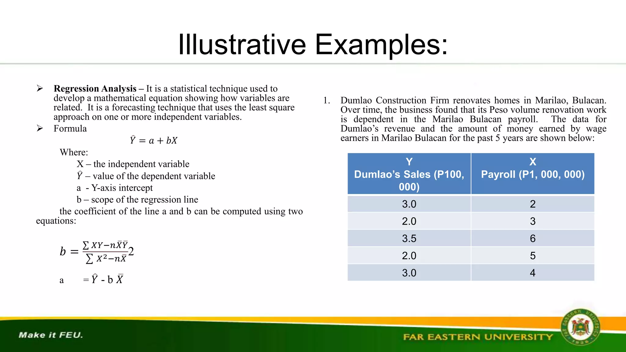
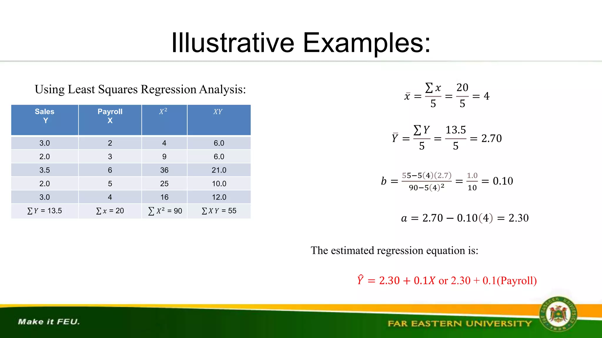
Here are 3 practice problems using quantitative forecasting methods: 1. Using simple exponential smoothing, forecast next period's sales given the following data with a smoothing constant of 0.3: Period: Sales 1: 100 2: 110 3: 120 4: ? Forecast: F1 = 100 F2 = 100 + 0.3(110 - 100) = 103 F3 = 103 + 0.3(120 - 103) = 108.9 F4 = 108.9 + 0.3(120 - 108.9) = 113.67 2. Using linear regression, forecast next year's profits based on advertising expenditures given: Year: Prof

1. Forecasting
Chapter 3

2. Forecasting
 It is the art and science of
predicting future event.
 Business Forecasting – is an
estimate or prediction of future
developments in business such as
sales, expenditures, revenues etc.
 One of the most important aspect in
corporate planning.
 Demand Forecasting – is a forecast
that predicts company sales.
1. Techniques assume some underlying causal
system that existed in the past will persist into
the future
2. Forecasts are not perfect
3. Forecasts for groups of items are more
accurate than those for individual items
4. Forecast accuracy decreases as the
forecasting horizon increases

3. Factors to consider:
Elements of a Good Forecast
The forecast
1. should be timely
2. should be accurate
3. should be reliable
4. should be expressed in meaningful units
5. should be in writing
6. technique should be simple to
understand and use
7. should be cost-effective
Steps in the Forecasting Process
1. Determine the purpose of the forecast
2. Establish a time horizon
3. Obtain, clean, and analyze appropriate
data
4. Select a forecasting technique
5. Make the forecast
6. Monitor the forecast errors

4. Forecast Accuracy Metrics
Mean Absolute Deviation
MAD weights all errors evenly
Mean Squared Error
MSE weights errors according to
their squared values
Mean Absolute Percent Error
MAPE weights errors according to
relative error
n
 
 t
t Forecast
Actual
MAD
 2
t
t
1
Forecast
Actual
MSE




n
n
 


100
Actual
Forecast
Actual
MAPE t
t
t

5. Forecast Error Calculation

6. Forecasting Methods:
Forecasting
Method
Quantitative
Methods
Time Series
Methods
Moving
Averages
Exponential
Smoothing
Trend
Projections
Causal
Methods
Regression
Analysis
Multiple
Regression
Qualitative
Methods
Delphi
Methods
Jury of
Executive
Opinions
Sales Force
Composite
Consumer
Market
Survey

7. Forecasting Approaches:
1. Qualitative Forecasting
– Forecasts that use subjective inputs
such as opinions from consumer
surveys, sales staff, managers,
executives, and experts
A. Judgmental Forecasts – rely on analysis of subjective inputs
obtained from various sources, such as consumer surveys, the sales staff,
managers, and executives, panels of experts etc.
B. Associative Model – forecasting technique that uses explanatory variables to
product future demand.
1. Executives Opinion – often used as a part of long-range planning and
new product development
2. Sales Force Composite – is a good source of information because of its
direct contrast with consumers
3. Consumer Surveys – It can tap information that might not be available
elsewhere
4. Outside Opinion – this may concern advice on political or economic
conditions is a foreign country or some other aspects of interest with
which an organization lacks familiarity
5. Opinions of Managers and Staff – At times, a manager may solicit from
a number of other managers and/or staff. The Delphi Method is useful
in this regard.

8. Forecasting Approaches:
2. Quantitative Forecast – time series – a time ordered
sequence of observations taken at regular intervals over
time. Plotting the data and visually examining the plot.
• Assume that future values of the time-series can be
estimated from past values of the time-series
- Trend – long term upward of downward movement in a data
1. Seasonal – short-term regular variations related to weather
or other factors
2. Cyclical – wavelike variation lasting more than one year
3. Irregular – variations caused by unusual circumstances not
by reflective or typical behavior
4. Random – residual variations after all other behaviors are
accounted for.
 Forecast based on Historical Data – a technique that
depends on uncovering relationships between variables
that can be used to predict future values of one of them.
 Averaging Technique – generate forecasts that reflect
recent values of a time-series
 Trend Line – associative to series of movements from a
straight line.
1. Naïve Forecast – a forecast for any period equals the previous
period’s actual value.
2. Moving Average – making use of the most recent data to get
the forecast.
3. Weighted Moving Average – weight can be used to place
more emphasis in recent values, when there is a trend or
pattern. This makes the technique more responsive to changes
since more recent period may be more heavily weighted.
4. Exponential Smoothing – Each new forecast is based on the
previous forecast plus a percentage of the difference between
that forecast and the actual value of the series at that point
5. Simple Linear Regression – the simple and most widely used
form of regression involves a linear relationship between two
variables. The objective in linear regression is to obtain an
equation of a straight line that minimizes the sum of equation
vertical deviations of points around the line.

9. Trend:

10. Illustrative Examples:
Averaging Techniques:
 Moving Average
Moving average =  Demand in previous n periods
n
Where:
n – is the number of period in the moving average
Compute a three-period moving average forecast given
the following demand for cars for the last five periods.
Week Demand
1 70
2 80
3 65
4 90
5 85
6 ?
80
85
83

11. Illustrative Examples:
 Weighted Moving Average
(weight for period n)(demand in period n)
 Weights
(weight for period n)(demand in period n)
= 85 .5 + 90 .3 + 65 .2
= 83(.5) + 85(.3) + 90(.2)
Compute for week 6 forecast using the weights: 50%,
30% and 20% respectively given the following demand
for cars for the last five periods.
83
85
84

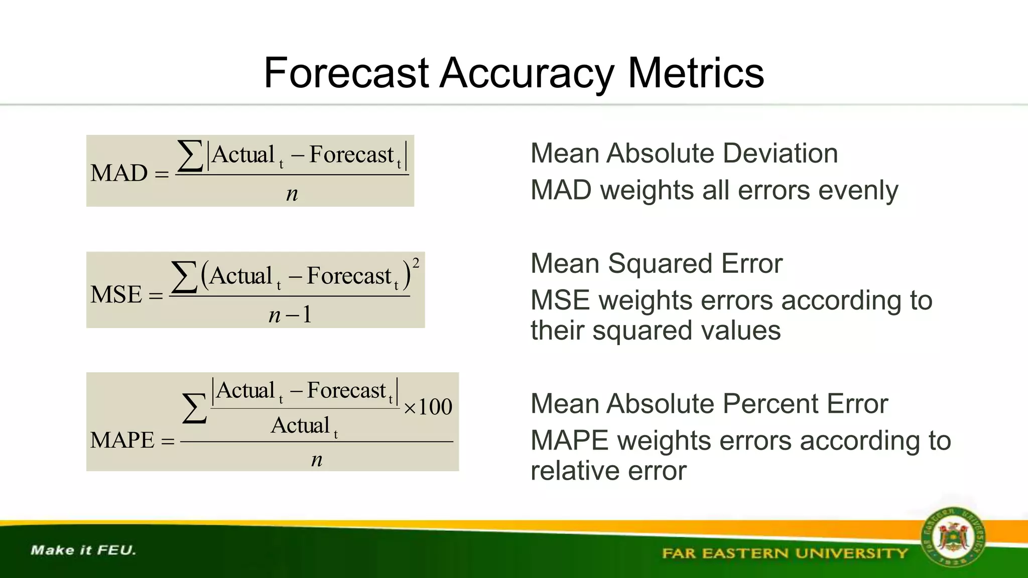
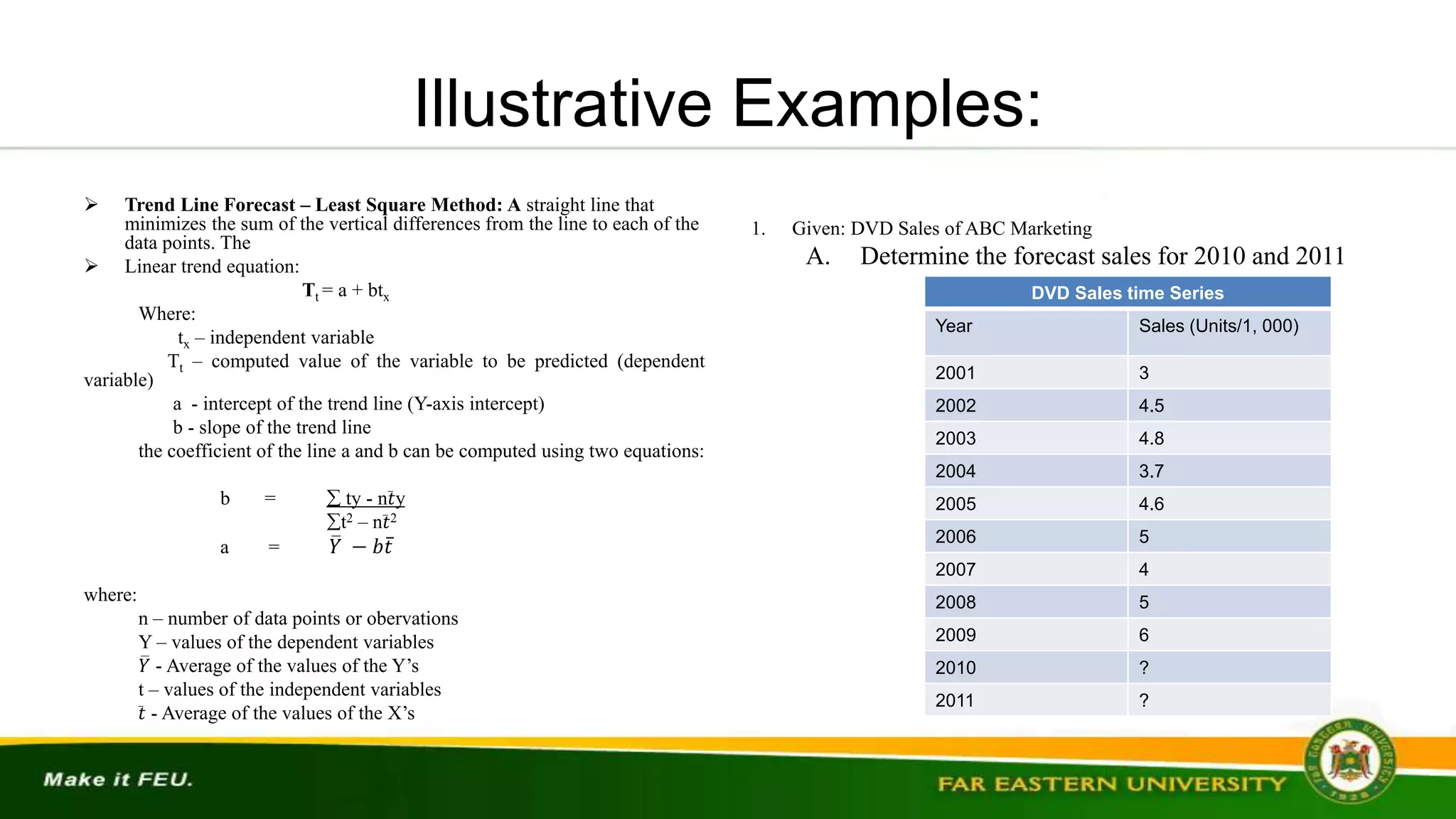
12. Illustrative Examples:
 Exponential Smoothing
 New forecast = Last Period’s Forecast +  (Last
Period’s Actual Demand – Last Period’s Forecast)
 Where:  represents the value of a weighing factor – smoothing
factor – value is 0 and 1.
Ft = Ft – 1 +  [At – 1 – Ft - 1]
Where:
Ft – the new forecast or forecast for period
Ft-1 – the previous forecast or forecast for period t-1
 - smoothing constant
At-1 – actual demand or sales for period t-1
 The smoothing constant, , represents percentage of the
forecast error. Each new forecast is equal to the
previous forecast plus a percentage of the previous
1. In January, a demand for 200 units of Toyota car model
“Vios” for February was predicted by a car dealer. Actual
February demand was 250 cars. Forecast the March
demand using a smoothing constant of  = 0.30.
New Forecast: 200 + 0.30(250-200) = 215 cars
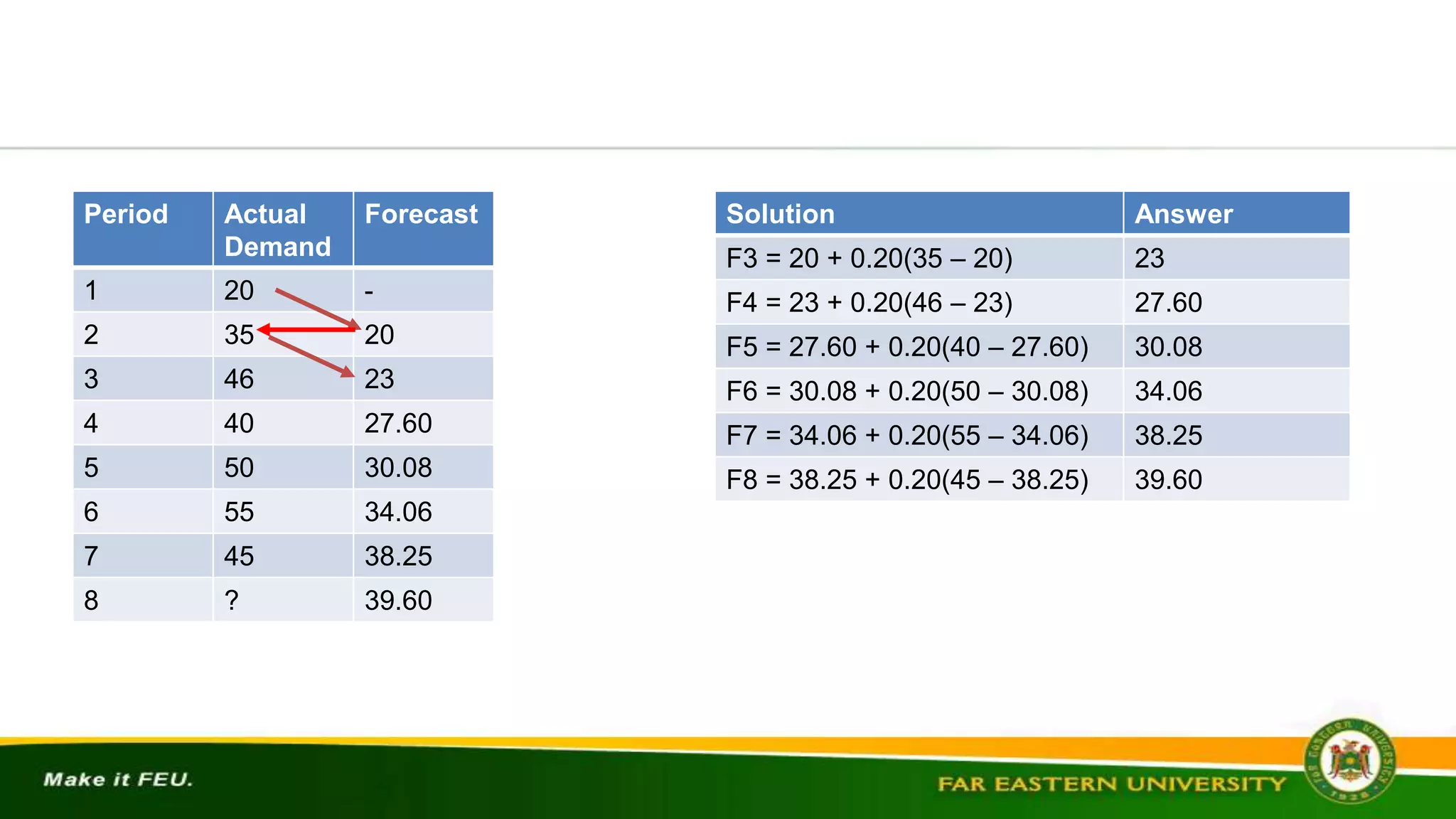
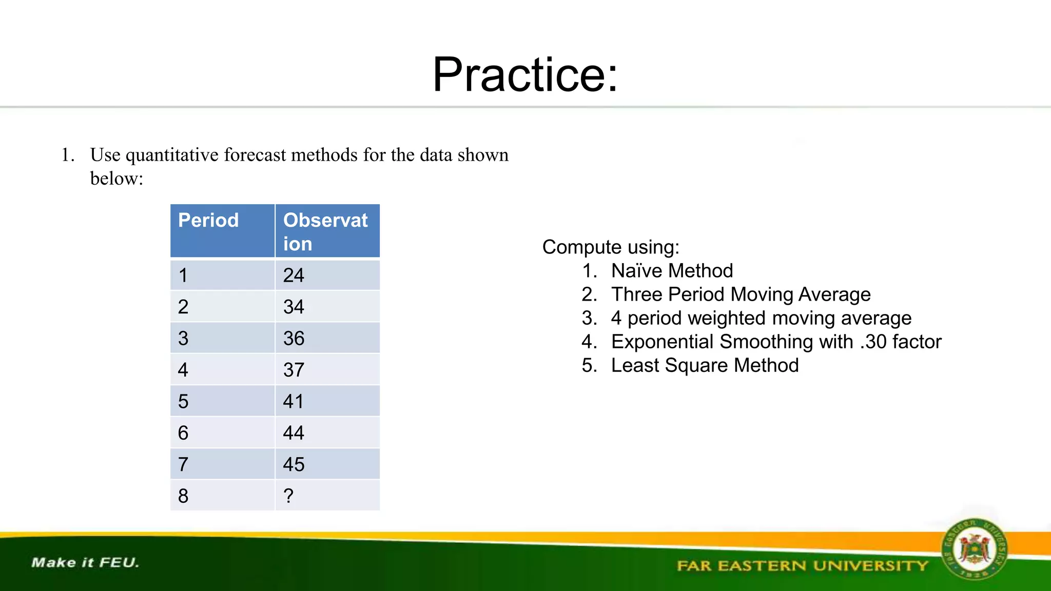
2. Use exponential smoothing model to develop a series of
forecast for the following data and compute.
a. Use a smoothing factor of 0.20
PERIOD ACTUAL DEMAND
1 20
2 35
3 46
4 40
5 50
6 55
7 45
8 ?

13. Period Actual
Demand
Forecast
1 20 -
2 35 20
3 46 23
4 40 27.60
5 50 30.08
6 55 34.06
7 45 38.25
8 ? 39.60
Solution Answer
F3 = 20 + 0.20(35 – 20) 23
F4 = 23 + 0.20(46 – 23) 27.60
F5 = 27.60 + 0.20(40 – 27.60) 30.08
F6 = 30.08 + 0.20(50 – 30.08) 34.06
F7 = 34.06 + 0.20(55 – 34.06) 38.25
F8 = 38.25 + 0.20(45 – 38.25) 39.60

14. Illustrative Examples:
 Trend Line Forecast – Least Square Method: A straight line that
minimizes the sum of the vertical differences from the line to each of the
data points. The
 Linear trend equation:
Tt = a + btx
Where:
tx – independent variable
Tt – computed value of the variable to be predicted (dependent
variable)
a - intercept of the trend line (Y-axis intercept)
b - slope of the trend line
the coefficient of the line a and b can be computed using two equations:
b =  ty - n𝑡y
t2 – n𝑡2
a = 𝑌 − 𝑏𝑡
where:
n – number of data points or obervations
Y – values of the dependent variables
𝑌 - Average of the values of the Y’s
t – values of the independent variables
𝑡 - Average of the values of the X’s
1. Given: DVD Sales of ABC Marketing
A. Determine the forecast sales for 2010 and 2011
DVD Sales time Series
Year Sales (Units/1, 000)
2001 3
2002 4.5
2003 4.8
2004 3.7
2005 4.6
2006 5
2007 4
2008 5
2009 6
2010 ?
2011 ?

15. Illustrative Examples:
Solutions:
𝑡 =
𝑡
𝑛
=
45
9
= 5 ; 𝑌 =
𝛴𝑌
𝑛
=
40.60
9
= 4.51
𝑏 =
216.20 − 9 5 4.51
285 − 9 5 2
𝑏 =
13.25
60
= 0 ⋅ 22
𝑎 = 4.51 − 0.22 5 = 3.41
The Trend Equation will be:
𝑇𝑡 = 3.41 + 0.22𝑡
DVD Sales time Series
Year Period
t
Sales (1, 000)
Y
𝑡2
ty
2001 1 3 1 3
2002 2 4.5 4 9
2003 3 4.8 9 14.4
2004 4 3.7 16 14.8
2005 5 4.6 25 23
2006 6 5 36 30
2007 7 4 49 28
2008 8 5 64 40
2009 9 6 81 54
𝑡 = 45 𝑌 = 40.6
𝑡2
= 285 𝑡𝑦 = 216.20

16. Illustrative Examples:
Sales forecast for 2010
𝑡𝑥 = 10
𝑇𝑡 = 3.41 + 0.22t
𝑇𝑡 = 3.41 + 0.22 10
𝑇10 = 3.41 + 2.2
𝑇10 = 5.61
Sales forecast for 2011
𝑡𝑥 = 11
𝑇𝑡 = 3.41 + 0.22 11
𝑇10 = 3.41 + 2.42
𝑇11 = 5.83

17. Illustrative Examples:
 Regression Analysis – It is a statistical technique used to
develop a mathematical equation showing how variables are
related. It is a forecasting technique that uses the least square
approach on one or more independent variables.
 Formula
𝑌 = 𝑎 + 𝑏𝑋
Where:
X – the independent variable
𝑌 – value of the dependent variable
a - Y-axis intercept
b – scope of the regression line
the coefficient of the line a and b can be computed using two
equations:
𝑏 =
𝑋𝑌−𝑛𝑋𝑌
𝑋2−𝑛𝑋
2
a = 𝑌 - b 𝑋
1. Dumlao Construction Firm renovates homes in Marilao, Bulacan.
Over time, the business found that its Peso volume renovation work
is dependent in the Marilao Bulacan payroll. The data for
Dumlao’s revenue and the amount of money earned by wage
earners in Marilao Bulacan for the past 5 years are shown below:
Y
Dumlao’s Sales (P100,
000)
X
Payroll (P1, 000, 000)
3.0 2
2.0 3
3.5 6
2.0 5
3.0 4

18. Illustrative Examples:
Using Least Squares Regression Analysis:
𝑥 =
𝑥
5
=
20
5
= 4
𝑌 =
𝑌
5
=
13.5
5
= 2.70
𝑏 =
55−5 4 2.7
90−5 4 2 =
1.0
10
= 0.10
𝑎 = 2.70 − 0.10 4 = 2.30
The estimated regression equation is:
𝑌 = 2.30 + 0.1𝑋 or 2.30 + 0.1(Payroll)
Sales
Y
Payroll
X
𝑋2
𝑋𝑌
3.0 2 4 6.0
2.0 3 9 6.0
3.5 6 36 21.0
2.0 5 25 10.0
3.0 4 16 12.0
𝑌 = 13.5 𝑥 = 20 𝑋2
= 90 𝑋 𝑌 = 55

19. Illustrative Examples:
 If Dumlao Construction wishes to have a payroll of
Php 5, 500, 000 next year, an estimated sales for
Dumlao Construction is:
Sales (P100, 000) = 2.30 + 0.1(Payroll)
= 2.30 + 0.1(5, 500, 000)
= 2.30 + 0.55
= 2.85
Sales = Php 2,850,000.00

20. Practice:
1. Use quantitative forecast methods for the data shown
below:
Period Observat
ion
1 24
2 34
3 36
4 37
5 41
6 44
7 45
8 ?
Compute using:
1. Naïve Method
2. Three Period Moving Average
3. 4 period weighted moving average
4. Exponential Smoothing with .30 factor
5. Least Square Method