Demand forecasting plays a key role in supply chain planning and decision making. Accurate forecasts are needed for production scheduling, inventory management, marketing activities, financial planning, and workforce management. However, forecasts are never perfectly accurate and error should be measured. Different forecasting techniques exist, including qualitative methods that use expert opinions and quantitative methods like time series analysis and regression. The bullwhip effect occurs when demand variability increases at each step up the supply chain, exacerbating distortions in information flow and potentially disrupting operations.

1. Demand Forecasting
1

2. Role of Forecasting
in a Supply Chain
• The basis for all strategic and planning decisions in a supply chain
• Used for both push and pull processes
• Examples:
– Production: scheduling, inventory, aggregate planning
– Marketing: sales force allocation, promotions, new production introduction
– Finance: plant/equipment investment, budgetary planning
– Personnel: workforce planning, hiring, layoffs
• All of these decisions are interrelated

3. Characteristics of Forecasts
• Forecasts are always wrong. Should include expected value and
measure of error.
• Long-term forecasts are less accurate than short-term forecasts
(forecast horizon is important)
• Aggregate forecasts are more accurate than disaggregate forecasts

4. Approaches to demand forecasting
• Understanding the objective of forecasting
• Integrate demand planning and forecasting throughout the
supply chain.
• Understanding and identifying customer segment.
• Identifying the major factors influence the demand forecast
• Determine the appropriate forecast technique
• Establish performance and error measures for forecasting.
4

5. COMPONENTS OF A FORECAST
• Past demand
• Lead time of product replenishment
• Planned advertising or marketing efforts
• Planned price discounts
• State of the economy
• Actions that competitors have taken
5

6. Types of Forecasts
6
Moving
Average
Exponential
Smoothing
Holt’s Model
Time-Series Methods: include
historical data over a time interval
Forecasting Techniques
No single method is superior
Delphi
Methods
Jury of Executive
Opinion
Sales Force
Composite
Consumer
Market Survey
Qualitative Models: attempt
to include subjective factors
Causal Methods: include a
variety of factors
Regression
Analysis
Multiple
Regression
Winter’s Model
Trend Projections

7. Qualitative Methods
Delphi Method
interactive group process consisting of obtaining information from
a group of respondents through questionnaires and surveys
Jury of Executive Opinion
obtains opinions of a small group of high-level managers in
combination with statistical models
Sales Force Composite
allows each sales person to estimate the sales for his/her region
and then compiles the data at a district or national level
Consumer Market Survey
solicits input from customers or potential customers regarding their
future purchasing plans
7

8. Decomposition of a Time-Series
Time series can be decomposed into:
 Trend (T): gradual up or down movement over time
 Seasonality (S): pattern of fluctuations above or below trend line that
occurs every year
 Cycles(C): patterns in data that occur every several years
 Random variations (R): “blips”in the data caused by chance and unusual
situations
 OBSERVED DEMAND = Systematic Component + Random
Component ( Forecast error)
8

9. Decomposition of Time-Series
The goal of any forecasting method is to predict the systematic
component of demand and estimate the random component. In
its most general form, the systematic component of demand
data contains a level, a trend, and a seasonal factor
Multiplicative model assumes demand is the product of
the four components
Demand = T * S * C * R
Additive model assumes demand is the summation of
the four components
Demand = T + S + C + R
9

10. Moving Averages
10
Simple moving average =
Moving average methods consist of computing an
average of the most recent n data values for the time
series and using this average for the forecast of the
next period.
 n
periods
n'
'
previous
in
demand

11. Three-Month Moving Average
11
Month Actual Shed
Sales
Three-Month
Moving Average
January 10
February 12
March 13
April 16
May 19
June 23
July 26
(10+12+13)/3 = 11 2/3
(12+13+16)/3 = 13 2/3
(13+16+19)/3 = 16
(16+19+23)/3 = 19 1/3

12. Weighted Moving Averages
12
Weighted moving averages use weights to put more
emphasis on recent periods.
Weighted moving average =

13. Weighted Moving Averages
13
Period
3 Last month
2 Two months ago
1 Three months ago
3*last month demand+2* two months ago demand+1*three months ago
demand
6 Sum of weights
Weights Applied

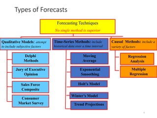
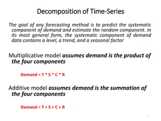
14. Weighted Three-Month Moving Average
14
Month Actual
Sales
Three-Month Weighted
Moving Average
10
12
13
16
19
23
January
February
March
April
May
June
July 26
[3*13+2*12+1*10]/6 = 12 1/6
[3*16+2*13+1*12]/6 =14 1/3
[3*19+2*16+1*13]/6 = 17
[3*23+2*19+1*16]/6 = 20 1/2

15. Exponential Smoothing
Exponential smoothing is a type of moving average
technique that involves little record keeping of past
data.
New forecast
= previous forecast + (previous actual –previous forecast)
Mathematically this is expressed as:
Ft = Ft-1 + (Dt-1 - Ft-1)
Ft-1 = previous forecast
 = smoothing constant (0<  <1)
Ft = new forecast
Dt-1 = previous period actual

16. Exponential Smoothing
Qtr Actual Rounded Forecast using  =0.10
1 180 175
2 168 175.00+0.10(180-175)= 175.5
3 159 175.50+0.10(168-175.50)= 174.75
4 175 174.75+0.10(159-174.75)= 173.18
5 190 173.18+0.10(175-173.18)= 173.36
6 205 173.36+0.10(190-173.36)= 175.02
7 180 175.02+0.10(205-175.02)= 178.02
8 182 178.02+0.10(180-178.02)=

17. Exponential Smoothing
Qtr Actual Tonnage
Unloaded
Rounded Forecast using  =0.50
1 180 175
2 168 175.00+0.50(180-175)= 177.50
3 159
4 175
5 190
6 205
7 180
8 182
9 ?

18. Exponential Smoothing with Trend
Adjustment( Holt’s model)
Simple exponential smoothing - first-order
smoothing
Trend adjusted smoothing - second-order
smoothing
Low  gives less weight to more recent trends,
while high  gives higher weight to more recent
trends.
Simple exponential smoothing fails to respond to trends, so
a more complex model is necessary with trend adjustment.

19. Exponential Smoothing with Trend
Adjustment( Holt’s model)
Forecast including trend (Ft+1)
= new forecast (Ft) + trend correction(Tt)
Ft =  Dt-1 +(1- )(Ft-1 + Tt-1)
Tt = (1 - )Tt-1 + (Ft – Ft-1)
where
Tt = smoothed trend for period t
Tt-1 = smoothed trend for the preceding period
 = trend smoothing constant
Ft = simple exponential smoothed forecast for period t
Ft-1 = forecast for period t-1

20. Example: Compute the adjusted exponential forecast for
the first week of march for a firm with the following data.
Assume the forecast for the first week of January (F0) as
600 and the corresponding initial trend (T0) as 0. let = 0.1
and =0.2.
20
Month
Jan. Feb.
Week 1 2 3 4 1 2 3 4
Demand 650 600 550 650 625 675 700 710

21. Solution: first week of jan.
Ft =  Dt-1 +(1- )(Ft-1 + Tt-1)
= 0.1 (650) + 0.9 (600 +0) = 605
Tt = (Ft – Ft-1)+ (1 - )Tt-1
= 0.2(605 - 600)+0.8(0)=1.00
Ft+1 = Ft + Tt = 605+1=606,
21

22. 22
So forecast for first week of march is 644.04, i.e 644 units.

23. Trend- and Seasonality-Corrected Exponential
Smoothing (Winter’s Model)
• Appropriate when the systematic component of demand is assumed to
have a level, trend, and seasonal factor
• Systematic component = (level+trend)(seasonal factor)
• Assume periodicity of demand to be p.
• Obtain initial estimates of level (L0), trend (T0), seasonal factors (S1,…,Sp)
using procedure for static forecasting
• In period t, the forecast for future periods is given by:
Ft+1 = (Lt+Tt)(St+1) and Ft+n = (Lt + nTt)St+n

24. Trend- and Seasonality-Corrected Exponential
Smoothing (continued)
After observing demand for period t+1, revise estimates for level,
trend, and seasonal factors as follows:
Lt+1 = (Dt+1/St+1) + (1-)(Lt+Tt)
Tt+1 = (Lt+1 - Lt) + (1-)Tt
St+p+1 = g(Dt+1/Lt+1) + (1-g)St+1
 = smoothing constant for level
 = smoothing constant for trend
g = smoothing constant for seasonal factor

25. Regression Analysis
In a simple regression analysis the relationship
between the dependent variable y and some
independent variable x can be represented by a
straight line
y= a+bx
Where, b is the slope of the line
a is the y-intercept
a = ∑y/ N
b = ∑xy/ ∑x2
25

26. Example: the following data gives the sales of the company for various
years. Fit the straight line. Forecast the sales for the year 2016.
26
year 2007 2008 2009 2010 2011 2012 2013 2014 2015
Sales
(000)
13 20 20 28 30 32 33 38 43

27. Year Sale (y) Deviation (x) x2 xy
1 13 -4 16 -52
2 20 -3 9 -60
3 20 -2 4 -40
4 28 -1 1 -28
5 30 0 0 0
6 32 1 1 32
7 33 2 4 66
8 38 3 3 114
9 43 4 16 172
N=9 ∑y= 257 ∑x=0 ∑x2 =60 ∑xy = 204
27
a = 28.56, b= 3.4
The equation of the straight line of best fit is
y= 28.56 + 3.4 x
So, sale for the year 2016 = 28.56 + 3.4 X 5 = 45.56= 45560

28. Forecasting Performance
• Mean Forecast Error (MFE or Bias): Measures average deviation of forecast
from actuals.
• Mean Absolute Deviation (MAD): Measures average absolute deviation of
forecast from actuals.
• Mean Absolute Percentage Error (MAPE): Measures absolute error as a
percentage of the forecast.
• Standard Squared Error (MSE): Measures variance of forecast error
How good is the forecast?
Forecast errors allow one to see how well the
forecast model works and compare that model with
other forecast models.

29. Measures of Forecast Accuracy
Forecast error = actual value – forecast value

30. Forecasting Performance Measures
)
(
1
1
t
n
t
t F
D
n
MFE 
 





n
t
t
t F
D
n
MAD
1
1




n
t t
t
t
D
F
D
n
MAPE
1
100
2
1
)
(
1
t
n
t
t F
D
n
MSE 
 


31. Mean Forecast Error (MFE or Bias)
• Want MFE to be as close to zero as possible -- minimum bias
• A large positive (negative) MFE means that the forecast is
undershooting the actual observations
• Note that zero MFE does not imply that forecasts are perfect
(no error) -- only that mean is “on target”
• Also called forecast BIAS
)
(
1
1
t
n
t
t F
D
n
MFE 
 


32. Mean Absolute Percentage Error
(MAPE)
• Same as MAD, except ...
• Measures deviation as a percentage of actual data




n
t t
t
t
D
F
D
n
MAPE
1
100

33. Mean Squared Error (MSE)
• Measures squared forecast error -- error variance
• Recognizes that large errors are disproportionately
more “expensive” than small errors
• But is not as easily interpreted as MAD, MAPE -- not as
intuitive
2
1
)
(
1
t
n
t
t F
D
n
MSE 
 


34. Tracking signal
• Should be within the range of +6
• Otherwise, possibly use a new forecasting method
TSt = bias / MADt
34

35. Hospital Days – Forecast Error Example
Ms. Smith forecasted
total hospital
inpatient days last
year. Now that the
actual data are
known, she is
reevaluating
her forecasting
model. Compute the
MAD, MSE, and
MAPE for her
forecast.
Month Forecast Actual
JAN 250 243
FEB 320 315
MAR 275 286
APR 260 256
MAY 250 241
JUN 275 298
JUL 300 292
AUG 325 333
SEP 320 326
OCT 350 378
NOV 365 382
DEC 380 396

36. Forecast Error – Example
Forecast Actual |error| error^2 |error/actual|
JAN 250 243 7 49 0.03
FEB 320 315 5 25 0.02
MAR 275 286 11 121 0.04
APR 260 256 4 16 0.02
MAY 250 241 9 81 0.04
JUN 275 298 23 529 0.08
JUL 300 292 8 64 0.03
AUG 325 333 8 64 0.02
SEP 320 326 6 36 0.02
OCT 350 378 28 784 0.07
NOV 365 382 17 289 0.04
DEC 380 396 16 256 0.04
MAD =
11.83
MSE =
192.83
MAPE = .0368*100
= 3.68

37. Bull Whip Effect in supply
chain
37

38. Whatis Bullwhip
!!
• Bullwhip effect is a phenomenon in forecast
driven distribution channels detected by
supply chain.
• In bullwhip effect order sent to the
manufacturer
and supplier create larger variance then the
sales to the end customers.

39. EffectsOfBullwhip
• In a supply chain plagued with Bullwhip effect,
the distortion in information is escalated as it
moves up in the chain.
• This variance can interrupt the smoothness of
the supply chain process as each link in the
supply chain will over or underestimate the
product demand i.e.
exaggerated fluctuations.

40. Symptoms of bullwhip
Some symptoms of Bullwhip
are:
• Excessive inventory
• Poor product forecast
• Insufficient capacities
• Long backlogs
• Uncertain Product planning

41. BULL
WHIP EFFECT E
X
A
M
P
L
E
CUSTOMER
0 20 40 60 80 100
120
RETAIL
ER
DISTRIBUT
OR
MANUFACTUR
ER
UNIT
S

42. BULL
WHIP EFFECT E
X
A
M
P
L
E
In the above example, the actual demand for customer is 10 units,the
retailer then orders 15 units from the distributor , an extra 5 units in
order to ensure they don’t run out of stock.
Then the supplier orders 40 units from manufacturer so that to buyin
bulk to ensure enough stock to provide timely shipment of goods to
retailer
The manufacturer then receives the order and it orders from their
supplier in bulk i.e. 100 units to ensure economy of sale in productionto
meet demand.
Now 100 units have produced to meet demand of 10 units which means
the retailer has to increase demand by dropping prices or finding more
customers that causes bullwhip effect.

43. BULL
WHIP EFFECT E
X
A
M
P
L
E

44. CA
USE
SOFBULL
WHIPEFFECT

45. Thank you
45