The document introduces concepts related to vector spaces including vectors, linear independence, and subspaces. It provides examples in R3 involving determining if sets of vectors are linearly dependent or independent, finding representations of vectors as linear combinations of other vectors, and solving homogeneous and nonhomogeneous systems of equations involving vector coefficients. Key concepts are illustrated through a series of problems involving vectors in R3.

1. SECTION 4.1
THE VECTOR SPACE R3
Here the fundamental concepts of vectors, linear independence, and vector spaces are introduced in
the context of the familiar 2-dimensional coordinate plane R2 and 3-space R3. The concept of a
subspace of a vector space is illustrated, the proper nontrivial subspaces of R3 being simply lines
and planes through the origin.
1. a − b = (2, 5, −4) − (1, −2, −3) = (1, 7, −1) = 51
2a + b = 2(2,5, −4) + (1, −2, −3) = (4,10, −8) + (1, −2, −3) = (5,8, −11)
3a − 4b = 3(2,5, −4) − 4(1, −2, −3) = (6,15, −12) − (4, −8, −12) = (2, 23, 0)
2. a − b = (−1, 0, 2) − (3, 4, −5) = (−4, −4, 7) = 81 = 9
2a + b = 2(−1, 0, 2) + (3, 4, −5) = (−2, 0, 4) + (3, 4, −5) = (1, 4, −1)
3a − 4b = 3(−1, 0, 2) − 4(3, 4, −5) = (−3, 0, 6) − (12,16, −20) = (−15, −16, 26)
3. a − b = (2i − 3j + 5k ) − (5i + 3 j − 7k ) = −3i − 6 j + 12k = 189 = 3 21
2a + b = 2(2i − 3j + 5k ) + (5i + 3 j − 7k )
= (4i − 6 j + 10k ) + (5i + 3j − 7k ) = 9i − 3j + 3k
3a − 4b = 3(2i − 3j + 5k ) − 4(5i + 3 j − 7k )
= (6i − 9 j + 15k ) − (20i + 12 j − 28k ) = − 14i − 21j + 43k
4. a − b = (2i − j) − ( j − 3k ) = 2i − 2 j + 3k = 17
2a + b = 2(2i − j) + ( j − 3k ) = (4i − 2 j) + ( j − 3k ) = 4i − j − 3k
3a − 4b = 3(2i − j) − 4( j − 3k ) = (6i − 3 j) − (4 j − 12k ) = 6i − 7 j + 12k
5. v = 3
2 u, so the vectors u and v are linearly dependent.
6. au + bv = a(0, 2) + b(3, 0) = (3b, 2a ) = 0 implies a = b = 0, so the vectors u and v
are linearly independent.
7. au + bv = a(2, 2) + b(2, −2) = (2a + 2b, 2a − 2b) = 0 implies a = b = 0, so the vectors
u and v are linearly independent.
8. v = − u, so the vectors u and v are linearly dependent.
In each of Problems 9-14, we set up and solve (as in Example 2 of this section) the system

2. u v1   a   w1 
au + bv =  1  b  = w  = w
u 2 v2     2
to find the coefficient values a and b such that w = au + bv,
 1 −1  a  1 
9.  −2 3   b  =  0  ⇒ a = 3, b = 2 so w = 3u + 2 v
    
3 2 a  0
10.  4 3   b  =  −1 ⇒ a = 2, b = −3 so w = 2u − 3v
    
5 2  a  1
11. 7 3   b  = 1 ⇒ a = 1, b = −2 so w = u − 2 v
   
 4 −2   a  2
12. 1 −1  b  =  −2  ⇒ a = 3, b = 5 so w = 3u + 5 v
    
7 3   a  5
13.  5 4   b  =  −2  ⇒ a = 2, b = −2 so w = 2u − 3v
    
 5 −6   a  5 
14.  −2 4   b  =  6  ⇒ a = 7, b = 5 so w = 7u + 5 v
    
In Problems 15-18, we calculate the determinant u v w so as to determine (using Theorem
4) whether the three vectors u, v, and w are linearly dependent (det = 0) or linearly
independent (det ≠ 0).
3 5 8
15. −1 4 3 = 0 so the three vectors are linearly dependent.
2 −6 −4
5 2 4
16. −2 −3 5 = 0 so the three vectors are linearly dependent.
4 5 −7
1 3 1
17. −1 0 −2 = − 5 ≠ 0 so the three vectors are linearly independent.
2 1 2

3. 1 4 3
18. 1 3 −2 = 9 ≠ 0 so the three vectors are linearly independent.
0 1 −4
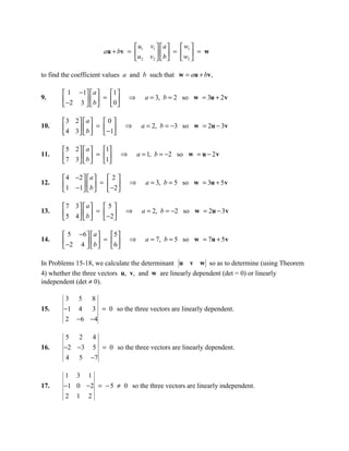
In Problems 19-24, we attempt to solve the homogeneous system Ax = 0 by reducing the
coefficient matrix A = [u v w ] to echelon form E. If we find that the system has only the
trivial solution a = b = c = 0, this means that the vectors u, v, and w are linearly independent.
Otherwise, a nontrivial solution x = [a b c ] ≠ 0 provides us with a nontrivial linear
T
combination au + bv + cw ≠ 0 that shows the three vectors are linearly dependent.
 2 −3 0   1 0 −3 
19.  0 1 −2  →  0 1 −2  = E
A =    
1 −1 −1
  0 0 0 
 
The nontrivial solution a = 3, b = 2, c = 1 gives 3u + 2v + w = 0, so the three vectors
are linearly dependent.
5 2 4 1 0 2 
20.  5 3 1  → 0 1 −3 = E
A =    
4 1 5 
  0 0 0 
 
The nontrivial solution a = –2, b = 3, c = 1 gives –2u + 3v + w = 0, so the three
vectors are linearly dependent.
 1 −2 3  1 0 11
21.  1 −1 7  → 0 1 4  = E
A =    
 −2 6 2 
  0 0 0 
 
The nontrivial solution a = 11, b = 4, c = –1 gives 11u + 4v – w = 0, so the three
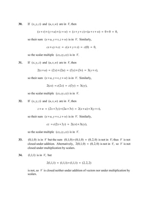
vectors are linearly dependent.
1 5 0  1 0 0 
22. 1 1 1  → 0 1 0  = E
A =    
0 3 2 
  0 0 1 
 
The system Ax = 0 has only the trivial solution a = b = c = 0, so the vectors u, v, and
w are linearly independent.
2 5 2  1 0 0 
23.  0 4 −1 →  0 1 0  = E
A =    
 3 −2 1 
  0 0 1 
 

4. The system Ax = 0 has only the trivial solution a = b = c = 0, so the vectors u, v, and
w are linearly independent.
1 4 −3 1 0 0
24.  4 2 3  → 0 1 0  = E
A =    
 5 5 −1
  0 0 1
 
The system Ax = 0 has only the trivial solution a = b = c = 0, so the vectors u, v, and
w are linearly independent.
In Problems 25-28, we solve the nonhomogeneous system Ax = t by reducing the augmented
coefficient matrix A = [u v w t ] to echelon form E. The solution vector
x = [a b c ] appears as the final column of E, and provides us with the desired linear
T
combination t = au + bv + cw.
1 3 1 2 1 0 0 2 
25.  −2 0 −1 −7  → 0 1 0 −1 = E
A =    
2 1 2 9
  0 0 1 3 
 
Thus a = 2, b = –1, c = 3 so t = 2u – v + 3w.
5 1 5 5  1 0 0 1 
26.  2 5 −3 30  → 0 1 0 5  = E
A =    
 −2 −3 4 −21
  0 0 1 −1
 
Thus a = 1, b = 5, c = –1 so t = u + 5v – w.
 1 −1 4 0  1 0 0 2 
27.  4 −2 4 0  → 0 1 0 6  = E
A =    
 3 2 1 19 
  0 0 1 1 
 
Thus a = 2, b = 6, c = 1 so t = 2u + 6v + w.
2 4 1 7  1 0 0 1
28.  5 1 1 7  → 0 1 0 1 = E
A =    
 3 −1 5 7 
  0 0 1 1
 
Thus a = 1, b = 1, c = 1 so t = u + v + w.
29. Given vectors (0, y , z ) and (0, v, w) in V, we see that their sum (0, y + v, z + w) and the
scalar multiple c(0, y, z ) = (0, cy, cz ) both have first component 0, and therefore are
elements of V.

5. 30. If ( x, y , z ) and (u , v, w) are in V, then
( x + v ) + ( y + u ) + ( z + w) = ( x + y + z ) + (u + v + w) = 0 + 0 = 0,
so their sum ( x + u , y + v, z + w) is in V. Similarly,
cx + cy + cz = c( x + y + x) = c(0) = 0,
so the scalar multiple (cx, cy, cz ) is in V.
31. If ( x, y , z ) and (u , v, w) are in V, then
2( x + u ) = (2 x) + (2u ) = (3 y ) + (3v) = 3( y + v),
so their sum ( x + u, y + v, z + w) is in V. Similarly,
2(cx) = c(2 x) = c(3 y ) = 3(cy ),
so the scalar multiple (cx, cy, cz ) is in V.
32. If ( x, y , z ) and (u , v, w) are in V, then
z + w = (2 x + 3 y ) + (2u + 3v) = 2( x + u ) + 3( y + v),
so their sum ( x + u , y + v, z + w) is in V. Similarly,
cz = c(2 x + 3 y ) = 2(cx) + 3(cy ),
so the scalar multiple (cx, cy, cz ) is in V.
33. (0,1, 0) is in V but the sum (0,1, 0) + (0,1, 0) = (0, 2, 0) is not in V; thus V is not
closed under addition. Alternatively, 2(0,1, 0) = (0, 2, 0) is not in V, so V is not
closed under multiplication by scalars.
34. (1,1,1) is in V, but
2(1,1,1) = (1,1,1) + (1,1,1) = (2, 2, 2)
is not, so V is closed neither under addition of vectors nor under multiplication by
scalars.

6. 35. Evidently V is closed under addition of vectors. However, (0, 0,1) is in V but
(−1)(0, 0,1) = (0, 0, −1) is not, so V is not closed under multiplication by scalars.
36. (1,1,1) is in V, but
2(1,1,1) = (1,1,1) + (1,1,1) = (2, 2, 2)
is not, so V is closed neither under addition of vectors nor under multiplication by
scalars.
37. Pick a fixed element u in the (nonempty) vector space V. Then, with c = 0, the scalar
multiple cu = 0u = 0 must be in V. Thus V necessarily contains the zero vector 0.
38. Suppose u and v are vectors in the subspace V of R3 and a and b are scalars. Then
au and bv are in V because V is closed under multiplication by scalars. But then it
follows that the linear combination au + bv is in V because V is closed under addition
of vectors.
39. It suffices to show that every vector v in V is a scalar multiple of the given nonzero
vector u in V. If u and v were linearly independent, then — as illustrated in Example
2 of this section — every vector in R2 could be expressed as a linear combination of u
and v. In this case it would follow that V is all of R2 (since, by Problem 38, V is closed
under taking linear combinations). But we are given that V is a proper subspace of R2,
so we must conclude that u and v are linearly dependent vectors. Since u ≠ 0, it
follows that the arbitrary vector v in V is a scalar multiple of u, and thus V is
precisely the set of all scalar multiples of u. In geometric language, the subspace V is
then the straight line through the origin determined by the nonzero vector u.
40. Since the vectors u, v, w are linearly dependent , there exist scalars p, q, r not all zero
such that pu + qv + rw = 0. If r = 0, then p and q are scalars not both zero such that
pu + qv = 0. But this contradicts the given fact that u and v are linearly independent.
Hence r ≠ 0, so we can solve for
p q
w = − u − v = au + b v ,
r r
thereby expressing w as a linear combination of u and v.
41. If the vectors u and v are in the intersection V of the subspaces V1 and V2, then
their sum u + v is in V1 because both vectors are in V1, and u + v is in V2 because
both are in V2. Therefore u + v is in V, and thus V is closed under addition of
vectors. Similarly, the intersection V is closed under multiplication by scalars, and is
therefore itself a subspace.