Eigenvalues and eigenfunctions are key concepts in linear algebra. An eigenfunction is a function that when operated on by a linear operator produces a constant multiplied version of itself. The constant is the corresponding eigenvalue. Eigenvalues are the solutions to the characteristic polynomial of the linear operator. Eigenfunctions are not unique as any constant multiple of an eigenfunction is also an eigenfunction with the same eigenvalue. The spectrum of an operator is the set of all its eigenvalues.

1. The world of Eigenvalues-eigenfunctions
An operator A operates on a function and produces a
function.
For every operator, there is a set of functions which
when operated by the operator produces the same
function modified only multiplied by a constant
factor.
Such a function is called the eigenfunction of the
operator, and the constant modifier is called its
corresponding eigenvalue. An eigenvalue is just a
number: Real or complex.
A typical eigenvalue equation would look like
Ax = λ x
Here, the matrix or the operator A operates on a
vector (or a function) x producing an amplified or
reduced vector λx . Here the eigenvalue λbelongs to
eigenfunction x .
d
Suppose the operator is A = ( x dx ) . A operating on
d n
x n produces Ax = x x = nx .
n n
dx

2. Therefore, the operator A has an eigenvalue n
corresponding to eigenfunction x n .
1. Eigenfunctions are not unique.
Suppose Ax = λ x . Define, another vector z = cx , where
c is a constant.
Now, Az = Acx = cAx = cλ x = λ cx = λ z
Therefore, z is also an e-function (eigenfunction)
of A.
2. If Ax = λ x is an eigenvalue equation (and we
assume that x is not a zero vector), then
Ax = λx ⇔ (A - λI)x = 0 ⇐⇒ det(A - λI) = 0
This leads to a characteristic polynomial in λ:
p A = det( A − λ I )
λ is an e-value of A only if pA = 0.
3. Spectrum of an operator A is σ( A ) : set of all its
e-values.
4. Spectral radius of an operator A is
ρ ( A ) = max | λ |
λ∈σ ( A ) = 1maxn | λi |
≤i ≤
5. Computation of spectrum and spectral radius:

3. 2 −1
Let A = 2 5  be the matrix and we want to
 
compute its eigenvalues and eigenfunctions. Its
characteristic equation (CE) is:
2 − λ −1 
det  = 0 ⇐⇒ (2 - λ )(5 - λ ) + 2 = 0
 2 5 − λ

This gives λ2 − 7λ + 12 = 0 ⇐ ⇒ ( λ − 3 )( λ − 4 ) = 0
Therefore, A has two eigenvalues: 3 and 4.
x 
Let the eigenfunction be the vector x =  1
 x2 
corresponding to e-value 3. Then
 2 − 1  x1   x1   3 x1 
 2 5   x  = 3 x  =  3 x 
  2   2   2 
Therefore, we have 2 x1 − x2 = 3x1 yielding
x1 = − x2 . Also, we get 2 x1 + 5 x2 = 3 x2 which gives us no new
result. Therefore, we can arbitrarily take the
1 
following solution: e1 = −1 corresponding to e-value 3
 
for the matrix A.

4. Similarly, for e-value of 4, the eigenfunction appears
1 
to be e2 = − 2 .
 
6. Faddeev-Leverrier Method to get characteristic
polynomial.
Define a sequence of matrices P = A, p1 = trace( P )
1 1
1
P2 = A[ P − p1I ] , p2 = trace( P2 )
1
2
1
P3 = A[ P2 − p2 I ] , p3 = trace( P3 )
3
…
…
1
Pn = A[ Pn −1 − pn −1I ] , p n = trace( Pn )
n
Then the characteristic polynomial P( λ ) is
[
P( λ ) = ( −1 )n λn − p1λn −1 − p2 λn − 2 − ... − pn ]
12 6 − 6
 6 16 2 
e.g. A=
 
− 6 2
 16 

Define P = A, p1 = trace( A ) = 12 + 16 + 16 = 44
1
P2 = A( P − p1I ) =
1
12 6 − 6− 32 6 −6 
 6 16 2  6 − 28 2 
  
− 6 2
 16  − 6
 2 − 28

− 312 −108 108 
= −108 − 408 − 60 , p 2 = −564
 
 108
 − 60 − 408


5. And one proceeds this way to get p3 = 1728
The CA polynomial = ( −1 )3 [λ3 − 44λ2 + 564λ −1728]
The eigenvalues are next found solving
[λ3 − 44λ2 + 564λ −1728] = 0
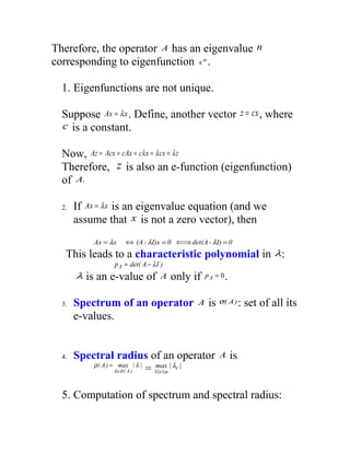
7. More facts about eigenvalues.
Assume Ax = λ x . Therefore, λ is the eigenvalue of
A with eigenvector x .
a. A−1 has the same eigenvector as A and the
corresponding eigenvalue is λ−1 .
b. An has the same eigenvector as A with the
eigenvalue λn .
c. ( A + µI ) has the same eigenvector as A with the
eigenvalue ( λ + µ ) .
d. If A is symmetric, all its eigenvalues are real.
e. If P is an invertible matrix then P −1 AP has the
same eigenvalues as A .
Proof of e.

6. Suppose, the eigenfunction of P −1 AP is y with
eigenvalue k .
Then,
P − APy = ky
1
⇐⇒ APy = Pky = kPy
Therefore, Py = x and k must be equal to λ. Therefore
the eigenvalues of A and P −1 AP are identical and the
eigenvector of one is a linear mapping of the other
one.
If the eigenvalues of A , λ1 ,λ2 ,...,λn are all distinct
then there exists a similarity transformation such that
λ1 0 0 .. 0 
0 λ 0 .. 0 
 2 
−1
P AP = D =  0 0 λ3 .. 0 
 .. .. .. .. 0 
 

0 0 0 .. λn 

Let the eigenvectors of A be x ( 1 ) , x ( 2 ) ,..., x ( i ) ,...x ( n )
such that we have Ax( i ) = λi x( i )
Then the matrix P = [ x( 1 ) , x( 2 ) ,..., x( n ) ]
Then AP = [ Ax( 1 ) , Ax( 2 ) ,..., Ax( n ) ]
[
= λ1 x( 1 ) ,λ2 x( 2 ) ,..., λn x( n ) ]
[ ][
= x ( 1 ) , x ( 2 ) ,..., x ( n ) λ1e( 1 ) ,λ 2 e( 2 ) ,..., λn e( n ) ]
= PD
Therefore, P −1 AP = D
Also, note the following. If A is symmetric, then

7. . So, we can normalize each
( x ( i ) )t x ( j)
= 0 , ∀i ≠ j
(i )
x (i)
eigenvector and obtain u = x so that the (i )
matrix Q = [u ( 1 ) ,u ( 2 ) ,...,u ( n ) ] would be an orthogonal matrix.
i.e. Q AQ = Dt
Matrix-norm.
Computationally, the l 2 -norm of a matrix is
determined as
l 2 -norm of [
A =|| A ||2 = ρ( At A ) ]1 / 2
1 1 0
e.g. A = 1 2 1
 
−1
 1 2

1 1 −1 1 1 0  3 2 −1
Then A A = 1
t
2 1  1 2 1 =  2 6 4
    
0
 1 2 −1
 1 2 −1
  4 5
The eigenvalues are:
λ1 = 0, λ2 = 7 + 7 , λ3 = 7 − 7
Therefore, A2 = ρ( At A ) = 7 + 7 ≈ 3.106
A ∞ = max ∑ aij
The l∞norm is defined as 1≤i ≤n j
1 1 0 
e.g. A =1 2 1 
 
−1
 1 − 4


8. 3 3
∑ a1 j = 1 + 1 + 0 = 2 , ∑ a2 j = 1 + 2 + 1 = 4
j =1 j =1
3
∑ a3 j = 6
j =1
Therefore, A ∞ = max( 2 ,4 ,6 ) = 6
In computational matrix algebra, we would often be
interested about situations when A k becomes small
(all the entrees become almost zero). In that case, A is
considered convergent.
is convergent if klim∞( A )ij = 0
k
i.e. A →
1 
 0
Example. Is A = 2 convergent?
1 1
 
4 2
1  1  1 
 4 0 8 0 16 0 
A2 =  A3 =  A4 = 
1 1 , 3 1 , 1 1 ,
     
 4 4 16 8   8 16 
It appears that
 1 
 2k 0
Ak = 
k 1
 
 2k + 1 2k 
 

9. 1
In the limit k → ∞,
2k
→0 . Therefore, A is a convergent
matrix.
Note the following equivalent results:
a. A is a convergent matrix
k
b1. klim∞ A 2 = 0
→
k
b2. klim∞ A ∞ = 0
→
c. ρ( A ) < 1
k
d. klim∞ A x = 0 ∀x
→
Condition number K( A ) of a non-singular matrix A
is computed as
K ( A ) = A . A -1
A matrix is well-behaved if its condition number is
close to 1. When K ( A ) of a matrix A is significantly
larger than 1, we call it an ill-behaved matrix.