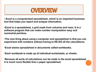
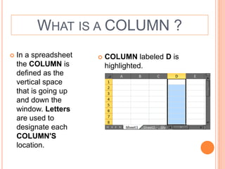
• Excel is a computerized spreadsheet, which is an important business
tool that helps you report and analyze information.
•Excel is a spreadsheet, a grid made from columns and rows. It is a
software program that can make number manipulation easy and
somewhat painless.
•The nice thing about using a computer and spreadsheet is that you can
experiment with numbers without having to RE-DO all the calculations.
•Excel stores spreadsheet in documents called workbooks.
•Each workbook is made up of individual worksheets, or sheets.
•Because all sorts of calculations can be made in the excel spreadsheet,
it is much more flexible than a paper spreadsheet.
OVERVIEW
 Spreadsheet
• A type of application program which manipulates numerical
and string data in rows and columns of cells.
 Workbook
• A booklet containing problems and exercises that a student
may work directly on the pages.
• A manual containing operating instructions, as for an
appliance or machine.
• A book in which a record is kept of work proposed or
accomplished.
 Worksheet
• A sheet of paper with multiple columns; used by an
accountant to assemble figures for financial statements.
• A piece of paper recording work planned or done on a project.
basics
 Spreadsheets are made up of
 Columns
 Rows
 and their intersections are called
cells
Basics of a Spreadsheet
WHAT IS A COLUMN ?
 In a spreadsheet
the COLUMN is
defined as the
vertical space
that is going up
and down the
window. Letters
are used to
designate each
COLUMN'S
location.
 COLUMN labeled D is
highlighted.
WHAT IS A ROW?
 In a spreadsheet
the ROW is
defined as the
horizontal space
that is going
across the
window.
Numbers are
used to designate
each ROW'S
location.
 ROW labeled 4 is
highlighted.
WHAT IS A CELL ?
 A CELL is the
space where a
row and column
intersect. Each
CELL is assigned
a name according
to its COLUMN
letter and ROW
number.
 In the above diagram
the CELL labeled C2 is
highlighted.
Identify Excel components
RIBBONS
 TABS:THERE ARE SEVEN TABS ACROSS THE TOP OF THE
EXCEL WINDOW.
 GROUPS: GROUPS ARE SETS OF RELATED
COMMANDS,DISPLAYED ON TABS.
 COMMANDS: A COMMAND IS A BUTTON,A MENU OR A BOX
WHERE YOU ENTER INFORMATION.
TABS
GROUPS
COMMANDS
Description of Excel
components
Data Tools
Excel 2010
 In each cell there may be the following data types:
 Labels -- (text with no numerical value)
 Number data -- (constant values)
 Formulas --(mathematical equation used to calculate)
TYPES OF DATA
Data Types Examples Descriptions
LABEL
Name or Wage or
Days
anything that is
just text
CONSTANT 5 or 3.75 or -7.4 any number
FORMULA =5+3 or = 8*5+3 math equation
Working with Data
 TO COPY AND PASTE CONTENTS:
 Select the cell or cells you wish to copy.
 Click the Copy command in the Clipboard group on the Home tab.
 Select the cell or cells where you want to paste the information.
 Click the Paste command.
 The copied information will now appear in the new cells
 TO CUT AND PASTE CELL CONTENTS:
 Select the cell or cells you wish to cut.
 Click the Cut command in the Clipboard group on the Home tab.
 Select the cell or cells where you want to paste the information.
 Click the Paste command.
 The cut information will be removed and now appear in the new cells.
 TO FORMAT TEXT IN BOLD, ITALICS OR UNDERLINE:
 Left-click a cell to select it or drag your cursor over the text in the formula bar to select it.
 Click the Bold, Italics or underline command.
 TO CHANGE THE FONT STYLE:
 Select the cell or cells you want to format.
 Left-click the drop-down arrow next to the Font Style box on the Home tab.
 Select a font style from the list.
Working with Data
 TO CHANGE THE FONT SIZE:
 Select the cell or cells you want to format.
 Left-click the drop-down arrow next to the Font Size box on the Home
tab.
 Select a font size from the list.
 TO ADD A BORDER:
 Select the cell or cells you want to format.
 Click the drop-down arrow next to the Borders command on the
Home tab. A menu will appear with border options.
 TO CHANGE THE TEXT COLOUR:
 Select the cell or cells you want to format.
 Left-click the drop-down arrow next to the Text Color command. A
color palette will appear.
 Select a color from the palette.
 TO ADD A FILL COLOUR:
 Select the cell or cells you want to format.
 Click the Fill command. A color palette will appear.
 Select a color from the palette.
CONDITIONAL FORMATTING
 TO APPLY CONDITIONAL
FORMATTING:
 Select the cells you would like to format.
 Select the Home tab.
 Locate the Styles group.
 Click the Conditional Formatting
command. A menu will appear with your
formatting options.
 TO REMOVE CONDITIONAL
FORMATTING:
 Click the Conditional Formatting
command.
 Select Clear Rules.
 Choose to clear rules from the entire
worksheet or the selected cells
CONDITIONAL FORMATTING
 TO APPLY NEW FORMATTING:
 Click the Conditional Formatting
command. Select New Rules from the
menu. There are different rules, you can
apply these rules to differentiate particular
cell.
 TO MANAGE CONDITIONAL
FORMATTING:
 Click the Conditional Formatting
command.
 Select Manage Rules from the menu.
The Conditional Formatting Rules
Manager dialog box will appear. From
here you can edit a rule, delete a rule, or
change the order of rules.
EDITING FILL
 In the lower right hand corner of the active cell
is excel’s “fill handle". When you hold your
mouse over the top of it, your cursor will turn
to a crosshair.
 If you have just one cell selected, if you click
and drag to fill down a column or across a row,
it will copy that number or text to each of the
other cells.
 If you have two cells selected, excel will fill in a
series. It will complete the pattern. For
example, if you put 4 and 8 in two cells select
them, click and drag the fill handle ,excel will
continue the pattern with 12,16,20.Etc.
 Excel can also auto- fill series of dates, times,
days of the week, months.
SORTING
 It means arranging data so
that it becomes easy to
analyze the data.
 You can sort the data
alphabetically, from highest
to lowest, or by a number of
additional criteria (such as
cell color).
CELL REFERENCING
A RELATIVE
CELL
REFERENCE
AS (A1) IS
BASED ON THE
RELATIVE
POSITION OF
THE CELL. IF
THE POSITION
OF THE CELL
THAT
CONTAINS THE
REFERENCE
CHANGES, THE
REFERENCE
ITSELF IS
CHANGED.
IN CELL (C1) SUM FUNCTION IS USED.
THEN FUNCTION FROM CELL (C1) IS COPY TO CELL (D3).
WHEN THE POSITION OF THE CELL IS CHANGED FROM (C1) TO
(D3),THEN THE REFERENCE IS ALSO CHANGED FROM (A1,B1) TO
(B3,C3).
CELL REFERENCING
AN ABSOLUTE
CELL
REFERENCE AS
($A$1) ALWAYS
REFERS TO A
CELL IN A
SPECIFIC
LOCATION. IF
THE POSITION
OF THE CELL
THAT CONTAINS
THE FORMULA
CHANGES, THE
ABSOLUTE
REFERENCE
REMAINS THE
SAME.
IN CELL (C1) SUM FUNCTION IS USED.
THEN FUNCTION FROM CELL (C1) IS COPY TO CELL (D3).
WHEN THE POSITION OF THE CELL IS CHANGED FROM (C1) TO
(D3),THEN THE ABSOLUTE REFERENCE REMAINS THE SAME(A1,B1).$
IS USED FOR CONSTANT ROW OR COLUMN.
Text To Column
 Text to Columns – delineate via special characters
or fixed width
Removing Duplicate Values
 Removing duplicate values – check for and delete
specific cells with duplicate values
Basic Formulas & Functions
Excel 2010
SUM FUNCTION
 Definition:
 Probably the most popular function in any spreadsheet
is the SUM function. The Sum function takes all of the
values in each of the specified cells and totals their
values.
 The syntax is: =SUM(first value, second value, etc) .
 => Text cells can not be added to a number and will
produce an error.
SUMIF FUNCTION
SYNTAX OF SUMIF
=SUMIF(RANGE,CRITERIA,SUM_RANGE)
RANGE-
Range of cells on which conditions
are applied.
CRITERIA-
Condition that defines which cell or
cells will be added.
SUM RANGE-
Actual cells to sum.
NOTE:-
If sum range is not used then range
is used for sum.WITHOUT
SUM_RANGE
=
=
AVERAGE FUNCTION
 The average function finds the average of the
specified data. (Simplifies adding all of the indicated
cells together and dividing by the total number of
cells.)
IF FUNCTION
oDefinition:
oThe IF function will check the
logical condition of a statement and
return one value if true and a
different value if false.
oThe syntax is:
=IF (condition, value-if-true, value-
if-false)
oThere are multiple ways to write
an IF statement to get the same
result
oIF Functions are like
programming - they provide
multiple answers based on certain
conditions.
DATEIF FUNCTION
=
=
=
=
=
=
SYNTAX OF DATEDIF
=DATEDIF(START_DATE,END_DATE,”INTERVAL”)
START DATE-
Date from which u want to calculate
difference.
END DATE-
Date up to which u want to calculate
difference.
INTERVAL-
Form in which u want to calculate
difference.
This says that I
am 19 years 6
months & 18
days old
“ D ” - D AY S
“ M ” - M O N T H S
“ Y ” - Y E A R S
“ Y M ” - M O N T H S O V E R Y E A R
“ M D ” - D AY S O V E R M O N T H
COUNT FUNCTION
 The Count function will return the number of entries
(actually counts each cell that contains NUMBER
DATA) in the selected range of cells.
 Remember: cell that are blank or contain text will not
be counted.
MAX & MIN FUNCTION
 The Max function will return the largest (max) value
in the selected range of cells.
 The Min function will display the smallest value in a
selected set of cells.
=MAX(B10:B12) =MIN(D10:D12)
CONCATENATE FUNCTION
oConcatenate function
- join several strings into
one text string
oNote: The
concatenate function
does not
automatically leave a
blank space between
words or other data.
OTHER FUNCTION
=
=
NOW RETURNS CURRENT DATE AND TIME.
TODAY RETURNS CURRENT DATE ONLY.
MOD RETURNS THE REMAINDER AFTER A
NO.
IS DIVIDED BY A DIVISOR.
LEN RETURNS THE NO. OF CHARACTERS
IN A
TEXT STRING.
SUM ADD ALL THE NUMBERS.
USES OF FUNCTIONS
=
=
=
EXCEL TABLES
Excel 2010
EXCEL TABLES
 To make managing and analyzing a
group of related data easier, you can turn
a range of cells into a Microsoft Office
Excel table (previously known as an
Excel list). A table typically contains
related data in a series of worksheet
rows and columns that have been
formatted as a table. By using the table
features, you can then manage the data
in the table rows and columns
independently from the data in other
rows and columns on the worksheet.
Creating a Table
Elements of an Excel Tables
 Header row By default, a table has a header row.
Every table column has filtering enabled in the header
row so that you can filter or sort your table data quickly.
Elements of an Excel Tables
Banded rows By default, alternate shading
or banding has been applied to the rows in a
table to better distinguish the data.
Elements of an Excel Tables
 Total row You can add a total row to your table that
provides access to summary functions (such as the
AVERAGE, COUNT, or SUM function). A drop-down list
appears in each total row cell so that you can quickly
calculate the totals that you want.
Useful Features
Excel 2010
Instantly Reveal Formulas And General Number
Format of all Cells
 Show all formulas and the general number format
of cells
 Saves you time because you don’t have to move
the cell pointer to check each formula one-by-one.
•Keyboard short cut to
Instantly reveal formulas
•press the Ctrl key and the tilde key at the same
time.
•To change your worksheet back to the normal view,
just press the Ctrl and tilde keys again
SET MARGINS
FILTERS
 The Filter is a quick and easy way to find and
work with a subset of data in a range of cells.
 Filtered data displays only the rows that meet
criteria (criteria: Conditions you specify to limit
which records are included in the result set of a
query or filter.) that you specify and hides rows
that you do not want displayed. After you filter
data, you can copy, find, edit, format, chart, and
print the subset of filtered data without
rearranging or moving it.
 You can also filter by more than one column.
 Using AutoFilter, you can create three types of
filters: by a list values, by a format, or by
criteria.
FREEZE HEADERS
 To freeze a row in your worksheet, highlight the
row where you wish all rows before the
highlighted row to be frozen or locked, go to
Window>Freeze Panes and you will see a line
appear across your worksheet. Everything
above the line is frozen and will remain in view
when you scroll down your worksheet.
SET PRINT AREA
FUNCTION AUDITING
SHOW ARROW THAT INDICATE WHAT
CELLS AFFECT THE VALUE OF THE
CURRENTLY SELECTED CELL.
IN THIS EXAMPLE CELLS A1 & A3 AFFECT
THE VALUE OF CELL C2 & CELLS A1 & A4
AFFECT THE VALUE OF CELL C6.
SHOW ARROW THAT INDICATE WHAT
CELLS ARE AFFECTED BY THE VALUE OF
THE CURRENTLY SELECTED CELL.
IN THIS EXAMPLE CELL C2 & C6 ARE
AFFECTED BY THE VALUE OF CELL A2
& CELL C6 IS ALSO AFFECTED BY THE
CELL A4.
TRACE PRECEDENTS
TRACE DEPENDENTS
SHORTCUT KEYS
SHORTCUT KEYS
 PARTICULARS
 EDIT THE ACTIVE CELL
 CREATE A CHART
 INSERT CELL COMMENT
 FUNCTION DIALOGUE BOX
 INSERT A NEW WORKSHEET
 CUT
 COPY
 PASTE
 HIDE THE SELECTED COLUMNS
 UNHIDE THE COLUMNS
 HIDE THE SELECTED ROWS
 UNHIDE THE ROWS
 SELECT ALL CELLS
 UNDO
 REDO
KEYS
F2
F11
SHIFT + F2
SHIFT + F3
SHIFT + F11
CTRL + X
CTRL + C
CTRL + V
CTRL + 0
CTRL + SHIFT + 0
CTRL + 9
CTRL + SHIFT + 9
CTRL + A
CTRL + Z
CTRL + Y
JAIPUR BRANCH OF ICAI

MIRCROSOFT EXCEL- brief and useful for beginners by RISHABH BANSAL

  • 2.
    • Excel isa computerized spreadsheet, which is an important business tool that helps you report and analyze information. •Excel is a spreadsheet, a grid made from columns and rows. It is a software program that can make number manipulation easy and somewhat painless. •The nice thing about using a computer and spreadsheet is that you can experiment with numbers without having to RE-DO all the calculations. •Excel stores spreadsheet in documents called workbooks. •Each workbook is made up of individual worksheets, or sheets. •Because all sorts of calculations can be made in the excel spreadsheet, it is much more flexible than a paper spreadsheet. OVERVIEW
  • 3.
     Spreadsheet • Atype of application program which manipulates numerical and string data in rows and columns of cells.  Workbook • A booklet containing problems and exercises that a student may work directly on the pages. • A manual containing operating instructions, as for an appliance or machine. • A book in which a record is kept of work proposed or accomplished.  Worksheet • A sheet of paper with multiple columns; used by an accountant to assemble figures for financial statements. • A piece of paper recording work planned or done on a project. basics
  • 4.
     Spreadsheets aremade up of  Columns  Rows  and their intersections are called cells Basics of a Spreadsheet
  • 5.
    WHAT IS ACOLUMN ?  In a spreadsheet the COLUMN is defined as the vertical space that is going up and down the window. Letters are used to designate each COLUMN'S location.  COLUMN labeled D is highlighted.
  • 6.
    WHAT IS AROW?  In a spreadsheet the ROW is defined as the horizontal space that is going across the window. Numbers are used to designate each ROW'S location.  ROW labeled 4 is highlighted.
  • 7.
    WHAT IS ACELL ?  A CELL is the space where a row and column intersect. Each CELL is assigned a name according to its COLUMN letter and ROW number.  In the above diagram the CELL labeled C2 is highlighted.
  • 8.
  • 9.
    RIBBONS  TABS:THERE ARESEVEN TABS ACROSS THE TOP OF THE EXCEL WINDOW.  GROUPS: GROUPS ARE SETS OF RELATED COMMANDS,DISPLAYED ON TABS.  COMMANDS: A COMMAND IS A BUTTON,A MENU OR A BOX WHERE YOU ENTER INFORMATION. TABS GROUPS COMMANDS
  • 10.
  • 11.
  • 12.
     In eachcell there may be the following data types:  Labels -- (text with no numerical value)  Number data -- (constant values)  Formulas --(mathematical equation used to calculate) TYPES OF DATA Data Types Examples Descriptions LABEL Name or Wage or Days anything that is just text CONSTANT 5 or 3.75 or -7.4 any number FORMULA =5+3 or = 8*5+3 math equation
  • 13.
    Working with Data TO COPY AND PASTE CONTENTS:  Select the cell or cells you wish to copy.  Click the Copy command in the Clipboard group on the Home tab.  Select the cell or cells where you want to paste the information.  Click the Paste command.  The copied information will now appear in the new cells  TO CUT AND PASTE CELL CONTENTS:  Select the cell or cells you wish to cut.  Click the Cut command in the Clipboard group on the Home tab.  Select the cell or cells where you want to paste the information.  Click the Paste command.  The cut information will be removed and now appear in the new cells.  TO FORMAT TEXT IN BOLD, ITALICS OR UNDERLINE:  Left-click a cell to select it or drag your cursor over the text in the formula bar to select it.  Click the Bold, Italics or underline command.  TO CHANGE THE FONT STYLE:  Select the cell or cells you want to format.  Left-click the drop-down arrow next to the Font Style box on the Home tab.  Select a font style from the list.
  • 14.
    Working with Data TO CHANGE THE FONT SIZE:  Select the cell or cells you want to format.  Left-click the drop-down arrow next to the Font Size box on the Home tab.  Select a font size from the list.  TO ADD A BORDER:  Select the cell or cells you want to format.  Click the drop-down arrow next to the Borders command on the Home tab. A menu will appear with border options.  TO CHANGE THE TEXT COLOUR:  Select the cell or cells you want to format.  Left-click the drop-down arrow next to the Text Color command. A color palette will appear.  Select a color from the palette.  TO ADD A FILL COLOUR:  Select the cell or cells you want to format.  Click the Fill command. A color palette will appear.  Select a color from the palette.
  • 15.
    CONDITIONAL FORMATTING  TOAPPLY CONDITIONAL FORMATTING:  Select the cells you would like to format.  Select the Home tab.  Locate the Styles group.  Click the Conditional Formatting command. A menu will appear with your formatting options.  TO REMOVE CONDITIONAL FORMATTING:  Click the Conditional Formatting command.  Select Clear Rules.  Choose to clear rules from the entire worksheet or the selected cells
  • 16.
    CONDITIONAL FORMATTING  TOAPPLY NEW FORMATTING:  Click the Conditional Formatting command. Select New Rules from the menu. There are different rules, you can apply these rules to differentiate particular cell.  TO MANAGE CONDITIONAL FORMATTING:  Click the Conditional Formatting command.  Select Manage Rules from the menu. The Conditional Formatting Rules Manager dialog box will appear. From here you can edit a rule, delete a rule, or change the order of rules.
  • 17.
    EDITING FILL  Inthe lower right hand corner of the active cell is excel’s “fill handle". When you hold your mouse over the top of it, your cursor will turn to a crosshair.  If you have just one cell selected, if you click and drag to fill down a column or across a row, it will copy that number or text to each of the other cells.  If you have two cells selected, excel will fill in a series. It will complete the pattern. For example, if you put 4 and 8 in two cells select them, click and drag the fill handle ,excel will continue the pattern with 12,16,20.Etc.  Excel can also auto- fill series of dates, times, days of the week, months.
  • 18.
    SORTING  It meansarranging data so that it becomes easy to analyze the data.  You can sort the data alphabetically, from highest to lowest, or by a number of additional criteria (such as cell color).
  • 19.
    CELL REFERENCING A RELATIVE CELL REFERENCE AS(A1) IS BASED ON THE RELATIVE POSITION OF THE CELL. IF THE POSITION OF THE CELL THAT CONTAINS THE REFERENCE CHANGES, THE REFERENCE ITSELF IS CHANGED. IN CELL (C1) SUM FUNCTION IS USED. THEN FUNCTION FROM CELL (C1) IS COPY TO CELL (D3). WHEN THE POSITION OF THE CELL IS CHANGED FROM (C1) TO (D3),THEN THE REFERENCE IS ALSO CHANGED FROM (A1,B1) TO (B3,C3).
  • 20.
    CELL REFERENCING AN ABSOLUTE CELL REFERENCEAS ($A$1) ALWAYS REFERS TO A CELL IN A SPECIFIC LOCATION. IF THE POSITION OF THE CELL THAT CONTAINS THE FORMULA CHANGES, THE ABSOLUTE REFERENCE REMAINS THE SAME. IN CELL (C1) SUM FUNCTION IS USED. THEN FUNCTION FROM CELL (C1) IS COPY TO CELL (D3). WHEN THE POSITION OF THE CELL IS CHANGED FROM (C1) TO (D3),THEN THE ABSOLUTE REFERENCE REMAINS THE SAME(A1,B1).$ IS USED FOR CONSTANT ROW OR COLUMN.
  • 21.
    Text To Column Text to Columns – delineate via special characters or fixed width
  • 22.
    Removing Duplicate Values Removing duplicate values – check for and delete specific cells with duplicate values
  • 23.
    Basic Formulas &Functions Excel 2010
  • 24.
    SUM FUNCTION  Definition: Probably the most popular function in any spreadsheet is the SUM function. The Sum function takes all of the values in each of the specified cells and totals their values.  The syntax is: =SUM(first value, second value, etc) .  => Text cells can not be added to a number and will produce an error.
  • 25.
    SUMIF FUNCTION SYNTAX OFSUMIF =SUMIF(RANGE,CRITERIA,SUM_RANGE) RANGE- Range of cells on which conditions are applied. CRITERIA- Condition that defines which cell or cells will be added. SUM RANGE- Actual cells to sum. NOTE:- If sum range is not used then range is used for sum.WITHOUT SUM_RANGE = =
  • 26.
    AVERAGE FUNCTION  Theaverage function finds the average of the specified data. (Simplifies adding all of the indicated cells together and dividing by the total number of cells.)
  • 27.
    IF FUNCTION oDefinition: oThe IFfunction will check the logical condition of a statement and return one value if true and a different value if false. oThe syntax is: =IF (condition, value-if-true, value- if-false) oThere are multiple ways to write an IF statement to get the same result oIF Functions are like programming - they provide multiple answers based on certain conditions.
  • 28.
    DATEIF FUNCTION = = = = = = SYNTAX OFDATEDIF =DATEDIF(START_DATE,END_DATE,”INTERVAL”) START DATE- Date from which u want to calculate difference. END DATE- Date up to which u want to calculate difference. INTERVAL- Form in which u want to calculate difference. This says that I am 19 years 6 months & 18 days old “ D ” - D AY S “ M ” - M O N T H S “ Y ” - Y E A R S “ Y M ” - M O N T H S O V E R Y E A R “ M D ” - D AY S O V E R M O N T H
  • 29.
    COUNT FUNCTION  TheCount function will return the number of entries (actually counts each cell that contains NUMBER DATA) in the selected range of cells.  Remember: cell that are blank or contain text will not be counted.
  • 30.
    MAX & MINFUNCTION  The Max function will return the largest (max) value in the selected range of cells.  The Min function will display the smallest value in a selected set of cells. =MAX(B10:B12) =MIN(D10:D12)
  • 31.
    CONCATENATE FUNCTION oConcatenate function -join several strings into one text string oNote: The concatenate function does not automatically leave a blank space between words or other data.
  • 32.
    OTHER FUNCTION = = NOW RETURNSCURRENT DATE AND TIME. TODAY RETURNS CURRENT DATE ONLY. MOD RETURNS THE REMAINDER AFTER A NO. IS DIVIDED BY A DIVISOR. LEN RETURNS THE NO. OF CHARACTERS IN A TEXT STRING. SUM ADD ALL THE NUMBERS. USES OF FUNCTIONS = = =
  • 35.
  • 36.
    EXCEL TABLES  Tomake managing and analyzing a group of related data easier, you can turn a range of cells into a Microsoft Office Excel table (previously known as an Excel list). A table typically contains related data in a series of worksheet rows and columns that have been formatted as a table. By using the table features, you can then manage the data in the table rows and columns independently from the data in other rows and columns on the worksheet.
  • 37.
  • 38.
    Elements of anExcel Tables  Header row By default, a table has a header row. Every table column has filtering enabled in the header row so that you can filter or sort your table data quickly.
  • 39.
    Elements of anExcel Tables Banded rows By default, alternate shading or banding has been applied to the rows in a table to better distinguish the data.
  • 40.
    Elements of anExcel Tables  Total row You can add a total row to your table that provides access to summary functions (such as the AVERAGE, COUNT, or SUM function). A drop-down list appears in each total row cell so that you can quickly calculate the totals that you want.
  • 41.
  • 42.
    Instantly Reveal FormulasAnd General Number Format of all Cells  Show all formulas and the general number format of cells  Saves you time because you don’t have to move the cell pointer to check each formula one-by-one. •Keyboard short cut to Instantly reveal formulas •press the Ctrl key and the tilde key at the same time. •To change your worksheet back to the normal view, just press the Ctrl and tilde keys again
  • 43.
  • 44.
    FILTERS  The Filteris a quick and easy way to find and work with a subset of data in a range of cells.  Filtered data displays only the rows that meet criteria (criteria: Conditions you specify to limit which records are included in the result set of a query or filter.) that you specify and hides rows that you do not want displayed. After you filter data, you can copy, find, edit, format, chart, and print the subset of filtered data without rearranging or moving it.  You can also filter by more than one column.  Using AutoFilter, you can create three types of filters: by a list values, by a format, or by criteria.
  • 45.
    FREEZE HEADERS  Tofreeze a row in your worksheet, highlight the row where you wish all rows before the highlighted row to be frozen or locked, go to Window>Freeze Panes and you will see a line appear across your worksheet. Everything above the line is frozen and will remain in view when you scroll down your worksheet.
  • 46.
  • 47.
    FUNCTION AUDITING SHOW ARROWTHAT INDICATE WHAT CELLS AFFECT THE VALUE OF THE CURRENTLY SELECTED CELL. IN THIS EXAMPLE CELLS A1 & A3 AFFECT THE VALUE OF CELL C2 & CELLS A1 & A4 AFFECT THE VALUE OF CELL C6. SHOW ARROW THAT INDICATE WHAT CELLS ARE AFFECTED BY THE VALUE OF THE CURRENTLY SELECTED CELL. IN THIS EXAMPLE CELL C2 & C6 ARE AFFECTED BY THE VALUE OF CELL A2 & CELL C6 IS ALSO AFFECTED BY THE CELL A4. TRACE PRECEDENTS TRACE DEPENDENTS
  • 48.
  • 49.
    SHORTCUT KEYS  PARTICULARS EDIT THE ACTIVE CELL  CREATE A CHART  INSERT CELL COMMENT  FUNCTION DIALOGUE BOX  INSERT A NEW WORKSHEET  CUT  COPY  PASTE  HIDE THE SELECTED COLUMNS  UNHIDE THE COLUMNS  HIDE THE SELECTED ROWS  UNHIDE THE ROWS  SELECT ALL CELLS  UNDO  REDO KEYS F2 F11 SHIFT + F2 SHIFT + F3 SHIFT + F11 CTRL + X CTRL + C CTRL + V CTRL + 0 CTRL + SHIFT + 0 CTRL + 9 CTRL + SHIFT + 9 CTRL + A CTRL + Z CTRL + Y
  • 50.