Very important documents

1. Introduction to Microsoft
Excel
1
Basic Computer skill training for Mattu University
Graduate Class of 2023 Students

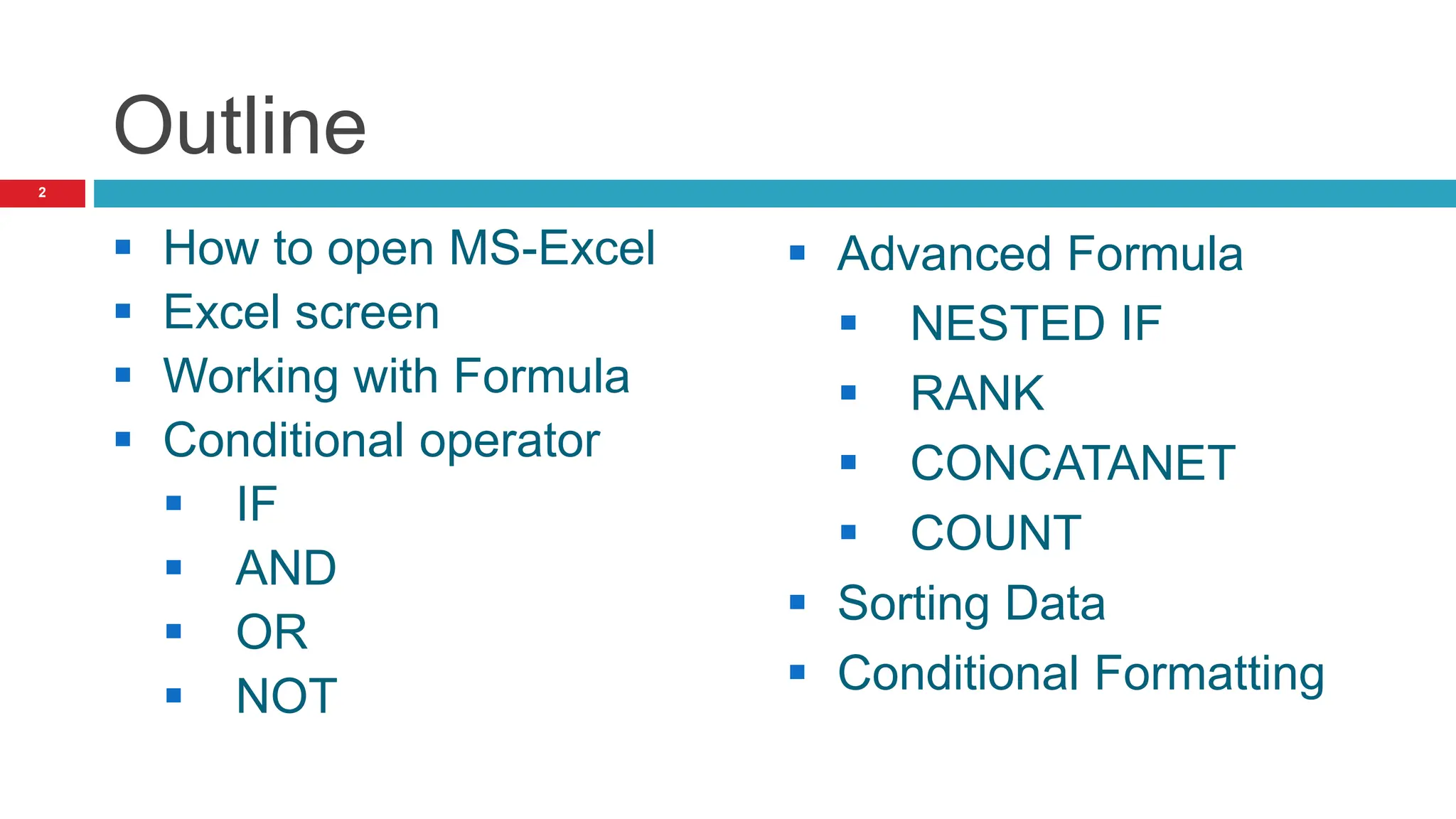
2. Outline
 How to open MS-Excel
 Excel screen
 Working with Formula
 Conditional operator
 IF
 AND
 OR
 NOT
 Advanced Formula
 NESTED IF
 RANK
 CONCATANET
 COUNT
 Sorting Data
 Conditional Formatting
2

3. How to open Microsoft Excel
3
• Follow these steps to run Excel from the Start menu.
• Step one: click on Start menu.
• Step two: Select All Programs from the pop-up menu.
• Step Three: Select Microsoft office
• Step Four: Select Microsoft Office Excel 2007 from the sub-
menu

4. How to open Microsoft Excel
4

5. The excel screen
5

6. Cont’d
6
Office Button which provides quick access for:
Creating
Opening
Saving
Printing
Preparing
Sending
Publishing and
Closing files.
 Recently accessed documents are also listed under this button.
 This button provides the only True menu within Excel 2007.

7. Cont’d
7
Save tool: used in order to save file
Undo: shows privies document
Minimizing: used to minimize document
Maximizing: used to maximize document
Closing: use to close program
 There is no way to delete or replace the Ribbon with the toolbars and menus
from previous versions of Microsoft Office.
 However, you can minimize the Ribbon to make more space available on the
screen.
 To quickly minimize the Ribbon, press (ctrl + F1).
• Use the Alt key to access the ribbon directly from the keyboard. For
example, if you were to press Alt+n, you could access the “Insert” Ribbon.
• Each time you press Alt, Excel displays corresponding letters for the Ribbon
items to help you to continue using keyboard shortcuts to select them.

8. Cont’d
8
Scroll bar used to quickly move (vertically) within your workbook.
Use the arrows located across the top and bottom of the scrollbar to move
up and down.
Column and Row
The next section across the top of the screen lists the columns and rows
within the current worksheet.
As mentioned, columns are lettered and rows are numbered.
The first 26 columns are lettered A through Z.
Excel then begins lettering the 27th column with AA and so on.
In a single Excel worksheet there are 16,384 columns (lettered A-XFD)
1,048,576 rows (numbered 1-1048576).

9. Cont’d
9
The outlined cell (the one with the dark borders) within the worksheet is referred to as
the active cell.
Each cell may contain text, numbers or dates.
You can enter up to 32,767 characters in each cell.
When you begin a new workbook, the tabs default to being labeled Sheet1, Sheet2,
etc.
Status Bar
 This bar is used to display various information about the system and current
workbook.
Mode Indicator
 which tells you what mode you are currently working in.
 When Excel is ready for you to enter text, the mode indicator will read “Ready”.
Zoom section
 Notice you can click on the increase or decrease buttons to change the zoom factor.

10. Cont’d
10
Changing the workbook view
By default, you are placed in “Normal” view which simply displays the worksheet.
However, if you’d prefer to see the headers, footers, and rulers you can switch to “Page Layout”
view.
Entering information
Excel allows you to type in words, numbers or formulas.
Click in the cell you want to store the data in and then simply begin typing the word(s), number or
formula.
If you make a mistake and want to start over, press Esc.
Notice as you type, the entry is displayed both in the cell and in the formula bar.
Editing data
If you type something in a cell and then decide later to change or correct it, place your pointer on
the cell to edit and reactivate it.
Double-Click on the cell you want to edit then type.

11. Cont’d
11
Deleting unwanted data
While pointing to the cell you want to clear, click the [RIGHT] mouse button once.
From the pop-up menu that appears, select cut.
Working with blocks
Many commands and operations require that you work on more than one cell at a time.
While you may not require the entire worksheet, you may need to work on a Block of cells.
Every block of cells has a beginning and ending address.
The beginning address is the address of the cell in the top-left corner of the block whereas the
ending address is the cell in the lower-right.
Mouse shapes
 thick cross, it can be used to select a single cell or block of cells for
editing purposes.
 diagonal arrow, you can move the contents of the currently selected cell or block of cells to
another location within the worksheet.
 thin cross-hair, you can fill a formula or other information into adjacent cells within the
worksheet.

12. Cont’d
12
Adjusting column width & row height
When entering large numbers, however, Excel will display the number in
scientific notation if the column is not wide enough to display the entire
number.
Should a cell be too narrow for text or numbers that you have entered, you
can widen the column in which the entry is located by following the steps
outlined below:
Place the mouse pointer in the column heading area to the right of the
lettered column to adjust.
Make sure the mouse pointer is on the column margin line.
The pointer changes to a cross-hair indicating you are on the margin line.
Click and drag the column margin line either to the right (expanding it) or to
the left (shrinking it).

13. Working with formula by excel
13
Formulas
A formula is a sequence of values, cell references, names, functions, or operators in a cell that together produce a new value.
A formula always begins with an equal sign (=).
Basic formula with its syntax
 To calculate the sum of a block of numbers, move to the cell where the answer is to be placed and use this function
argument:
=SUM (FIRST CELL:LAST CELL)
 You must define the block just like any other block by specifying the first and last cell addresses.
 To calculate the average value for a block of cells:
=AVERAGE (FIRST CELL: LAST CELL)
 To return the largest value in a block of cells:
=MAX (FIRST CELL: LAST CELL)
 To return the smallest value in a block of cells:
=MIN (FIRST CELL:LAST CELL)
 To count the number of numeric entries in a block of cells:
=COUNT (FIRST CELL:LAST CELL)

14. Conditional Operators
14
logical_test: The condition that you want to check.
value_if_true: The value to return if the condition is
True.
value_if_false: The value to return if the condition is
False
These formulas generally use the operators IF, AND, OR and NOT.
IF: function uses the following arguments:

15. 15

16. Cont’d
• Example: In the image below, the
logical test is whether the
student’s grade is greater than
75. If it is (in other words, the test
is true), then the cell will display
Pass. If it is false (less than 75),
the value will be displayed as
Fail.
• Note: If you want the formula to
display a text value, such as
Pass or Fail or A, B, C, D, etc,
you must put that text value in
quotation marks in the formula.
16

17. Cont’d
AND: returns TRUE if all of the
arguments are TRUE.
• Example: In the image below,
both test grades have to be
over 75 for the value in
column D to be true.
17

18. Cont’d
OR: returns TRUE if any of
the arguments are true.
• Example: In the image below,
if any of the test grades are
above 75 then the value in
column D will be TRUE. If
none of them are, the value
will be reflected as FALSE.
18

19. Cont’d
NOT: reverses the logic of its
argument.
• Example:
19

20. Advanced Formulas
20
Nested IF:
Excel can also use multiple formulas in the same cell.
For instance, you can nest multiple IF statements in one strand of logical
tests.
Example: In the image below, letter grades are calculated based on the
average final grade for each student and on a grade scale.
The nested IF formula follows the same template as before, however, in the
place of the “value if false” argument, you start the next IF statement
instead.

21. Cont’d
21
Note: You may put up to 64 nested IF statements in one formula.

22. Cont’d
RANK
• This function returns the rank
of a number amongst a list of
numbers.
• It does not reorder the cells;
rather it tells you where a
particular value falls in a
ranking of a specified range of
values.
• Example: The formula below
ranks the final grades in
descending order.
22

23. Cont’d
23
• The formula is specified as:
=RANK(cell, range, count by)
• Note: The range is an absolute reference so that as you copy the formula down it
does not change relative to the cell position.
CONCATENATE
 The CONCATENATE function joins up to 255 text strings into one text string. The
joined items can be text, numbers, cell references, or a combination of those items.
 For example, if your worksheet contains a person's first name in cell A1 and the
person's last name in cell B1, you can combine the two values in another cell by
using the following formula:
=CONCATENATE(A1," ",B1)
 The second argument in this example (" ") is a space character. You must specify
any spaces or punctuation that you want to appear in the results as an argument that
is enclosed in quotation marks.
• Example:

24. Cont’d
24

25. Cont’d
COUNT
 The COUNT function counts the
number of cells that contain
numbers, and counts numbers
within the list of arguments.
 Use the COUNT function to get
the number of entries in a
number field that is in a range or
array of numbers.
 For example, you can enter the
following formula to count the
numbers in the range A1:A20:
=COUNT(A1:A20)
25

26. Sorting data
 Sorting data is an integral part of analyzing
and organizing your information.
 For instance, if you have a listing of names
and addresses, you may want to sort by the
resident’s last name, or perhaps by zip
code.
 In Excel, you can sort text, numbers, dates
and other forms of information.
To sort data, regardless of the form, the first
step is to select the entire range of data
you want to sort.
 It is important to include all of the data so
that all of the data sorts together.
 On the home tab, click the Sort & Filter
button.
 You can sort in ascending (A-Z) or
descending (Z-A) order.
Example:
26

27. Conditional formatting
27
• Conditional formatting alters the appearance of your data
dependent on a set of rules that you designate. It is an easy
way to visually signify trends or outliers.
• First, select the cell(s) you wish to apply the rules to.
• Then, on the home tab, select Conditional Formatting.
• There are many options for applying the conditional
formatting, but one simple way is to select Highlight Cell
Rules.
• If you wish for the formatting to apply to values greater than a
specific number, select Greater than… .

28. Cont’d
• In the box that pops up, type in a
value.
• Values greater than (or less than,
depending on which option you
chose) will display the conditional
formatting.
• In the pull-down menu you can
choose which formatting to apply to
values that obey your rules.
• If you do not like the choices, you can
also choose Custom Format and
create a formatting style of your own.
• When you are finished, click OK.
28

29. Cont’d
29

30. Cont’d
30

31. Graphs and Charts
31
• Charts are used to display series of numeric data in a graphical
format to make it easier to understand large quantities of data and
the relationship between different series of data.
• Microsoft Excel 2007 no longer has the chart wizard present in
2003.
• Instead, it allows you to edit all parts of your chart easily from the
menu ribbon.
• To create a chart in excel, first select the range of data you would
like to include in the graph.
• Then, on the Insert ribbon, select the type of chart you prefer.

32. Cont’d
32

33. Thanks!
33