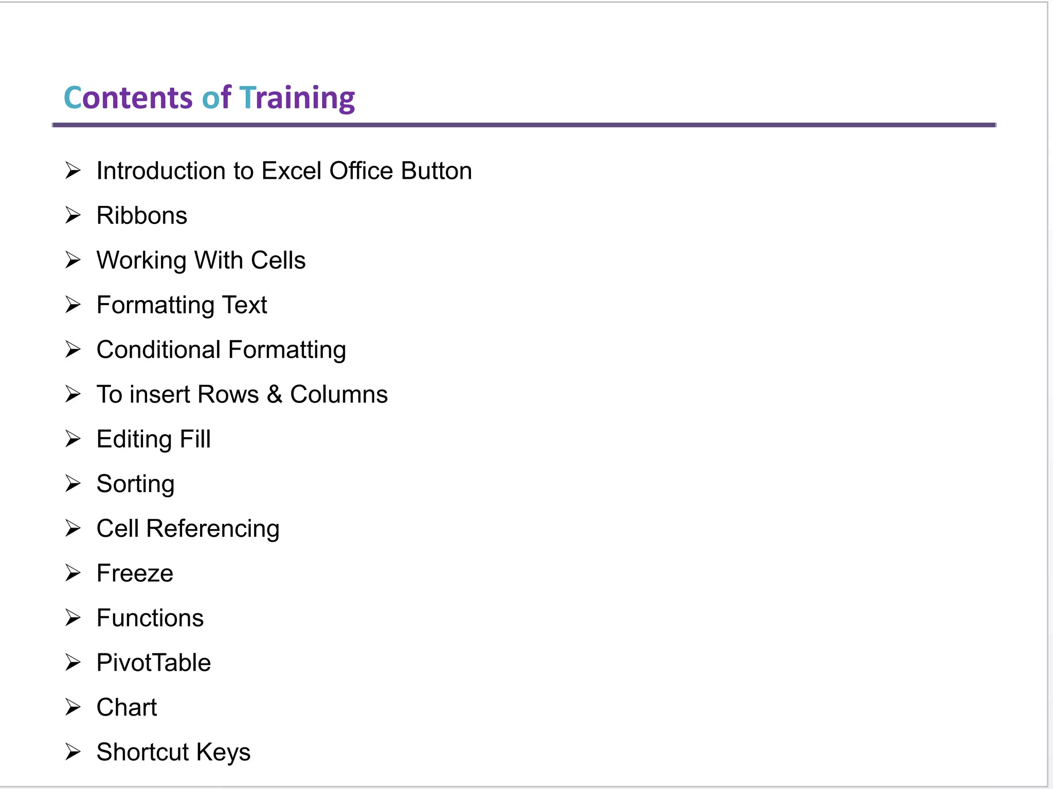
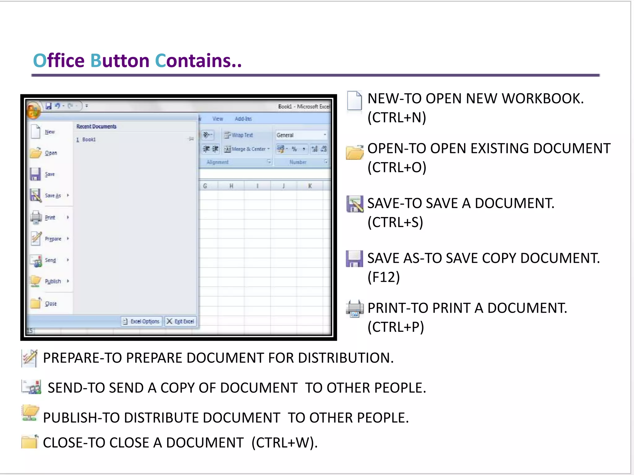
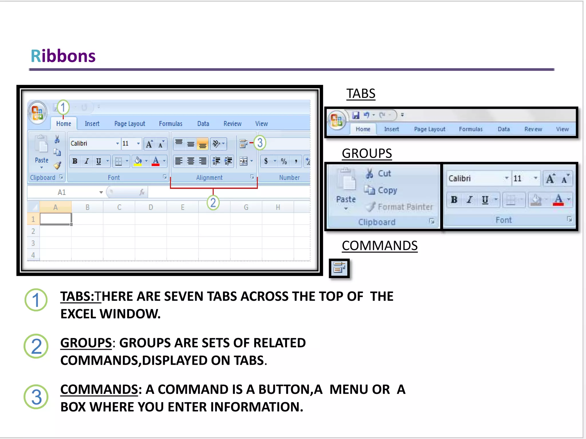
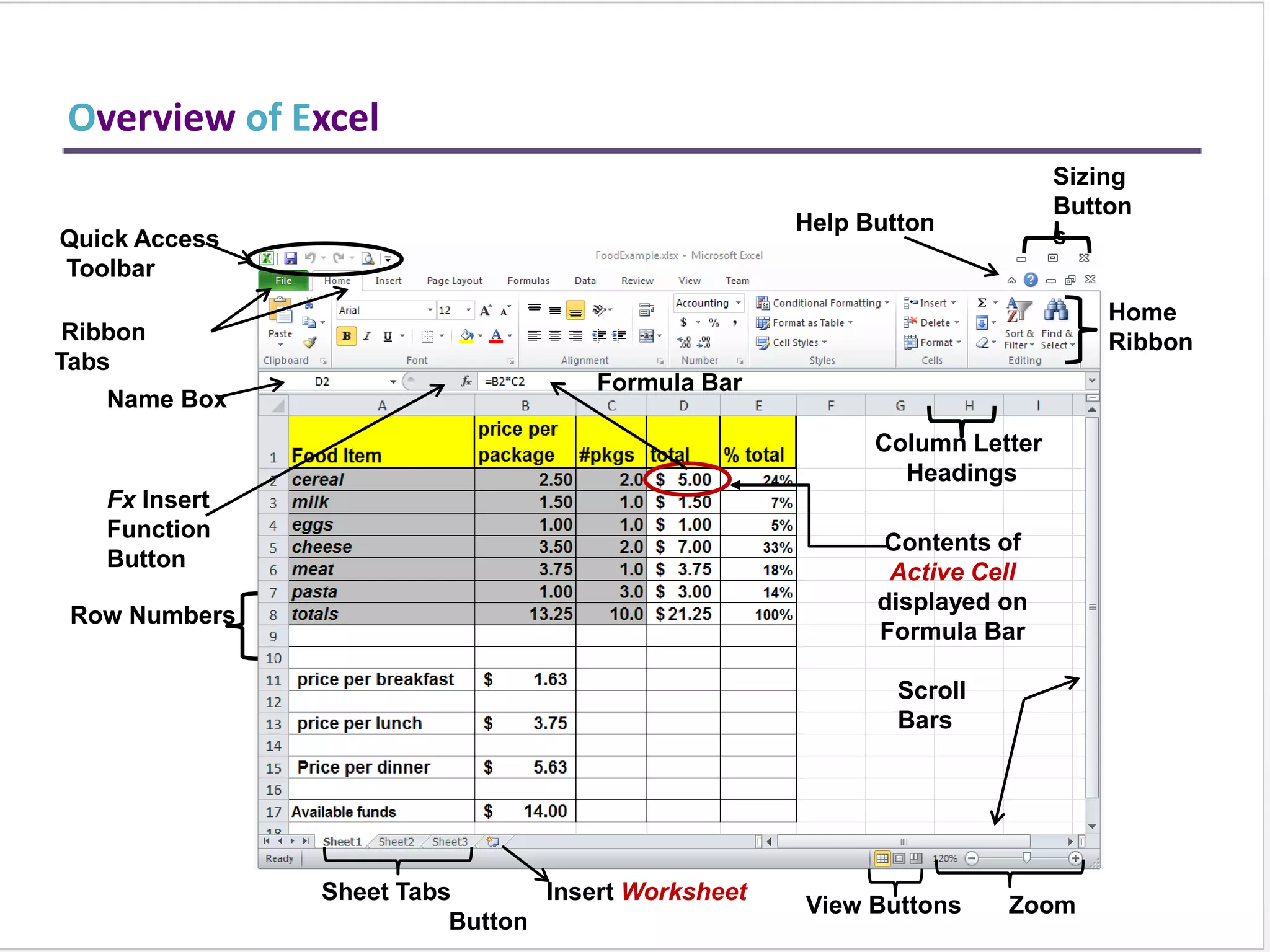
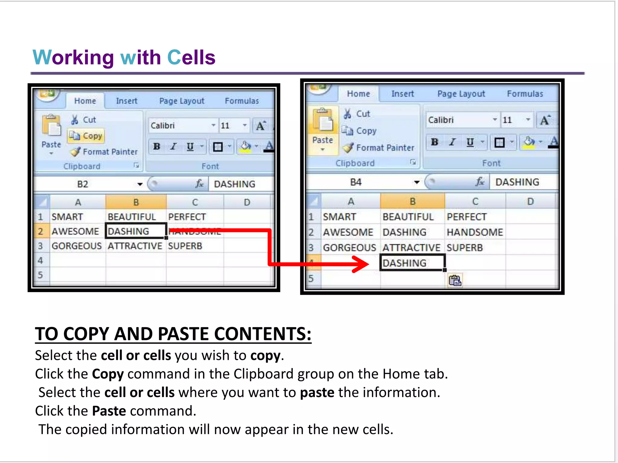
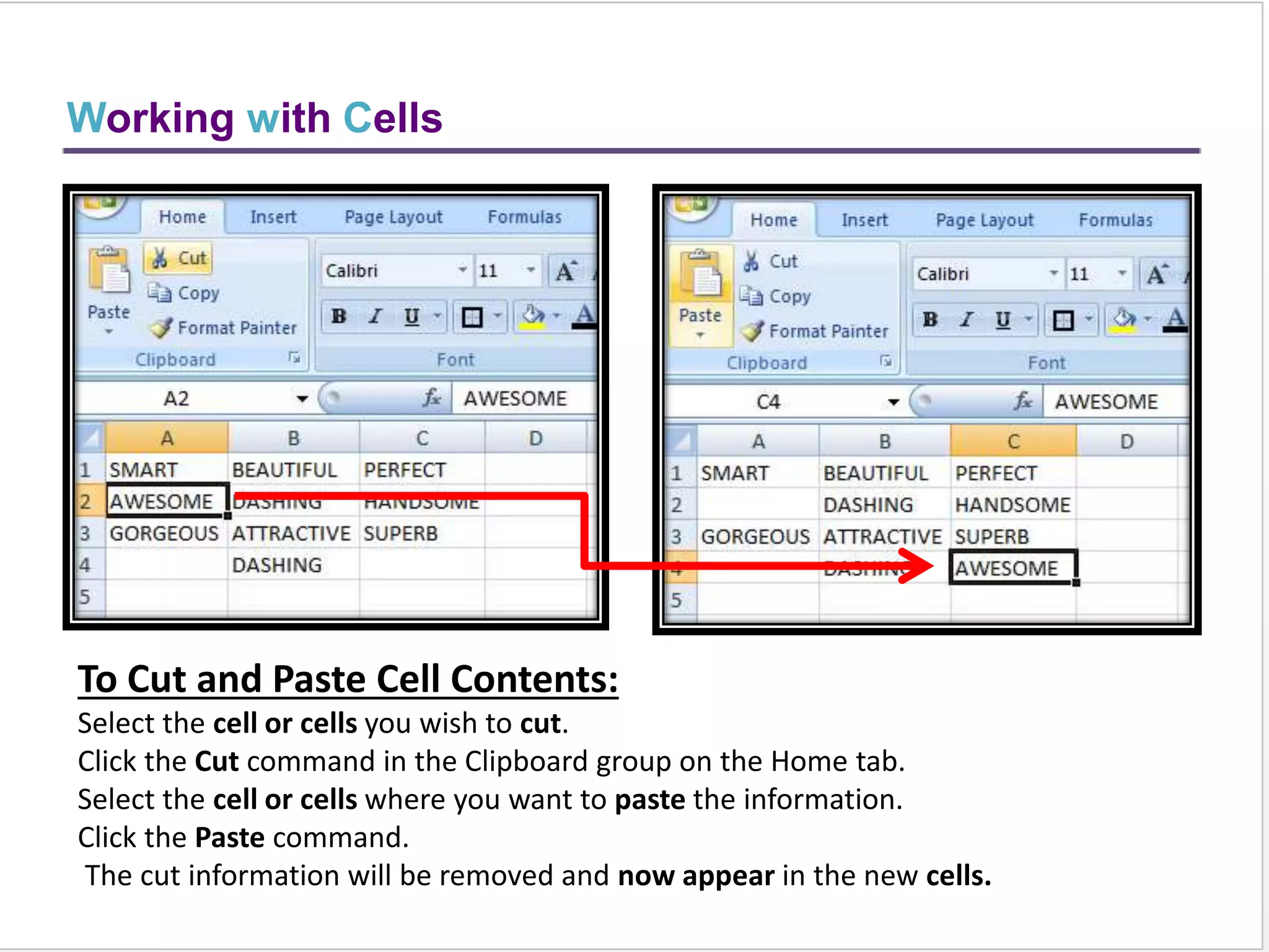
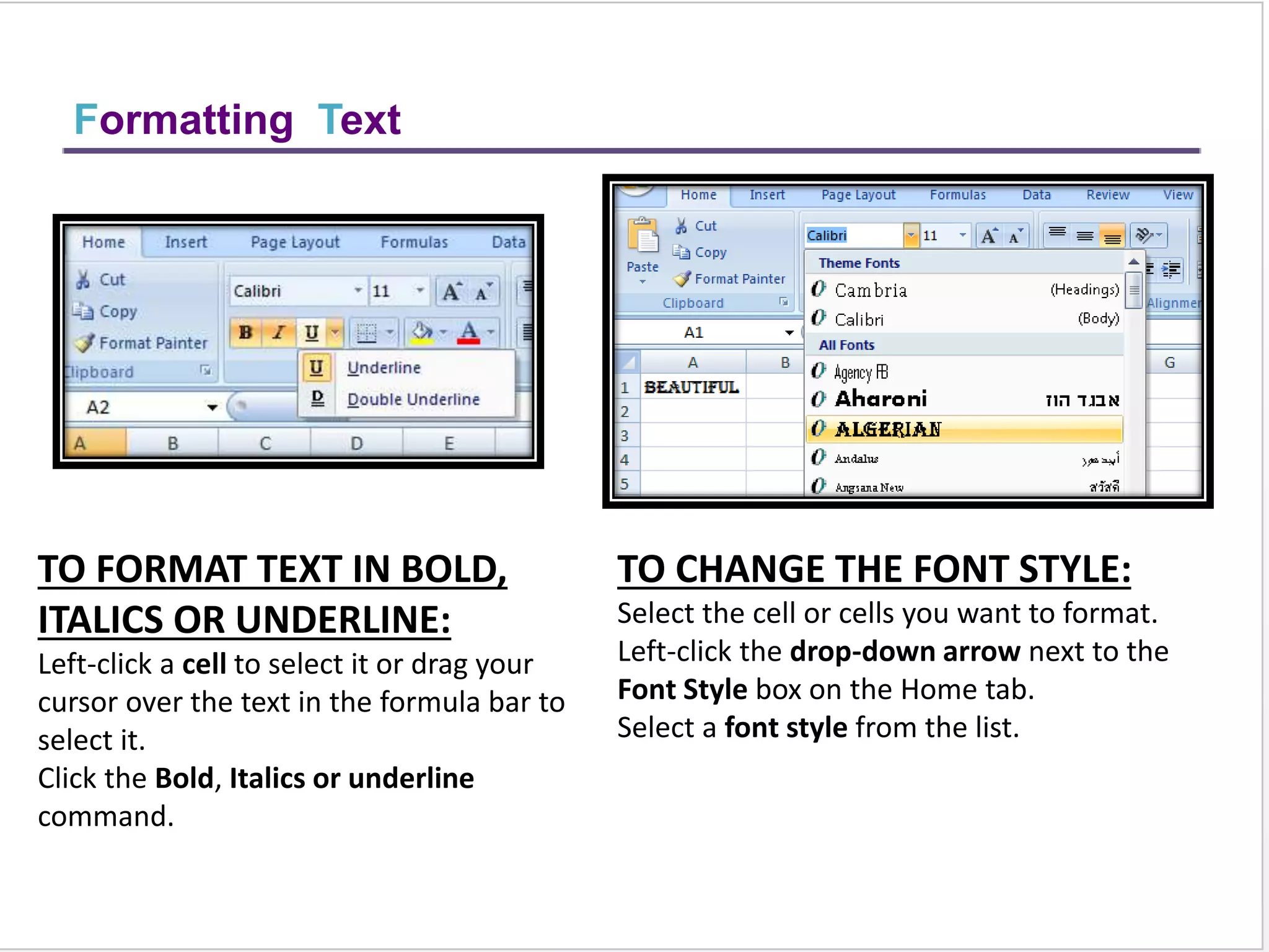
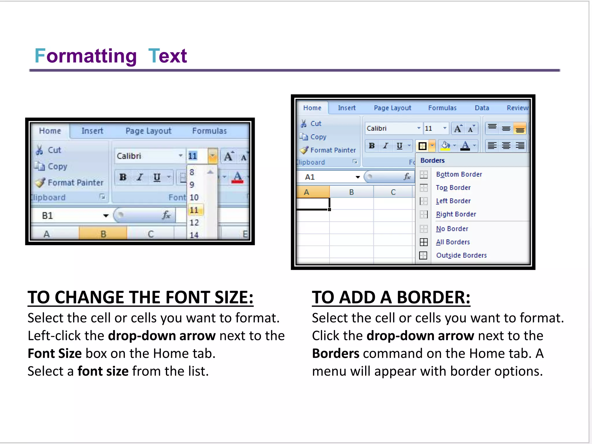
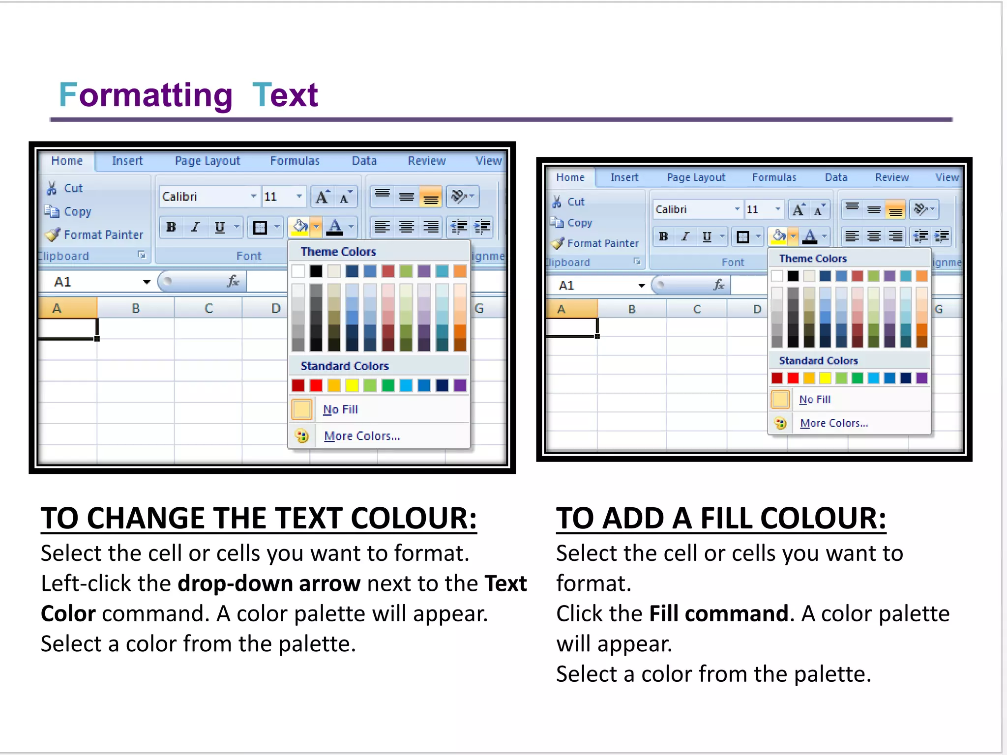
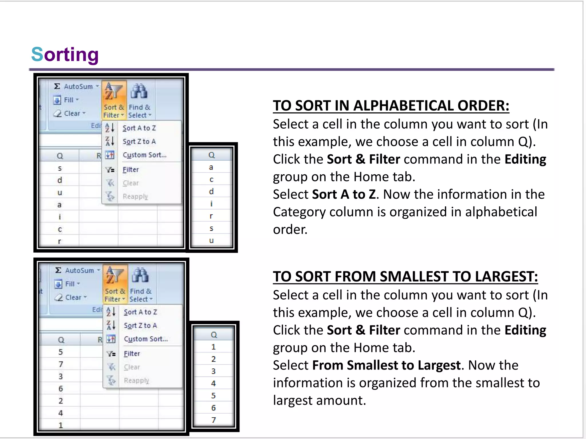
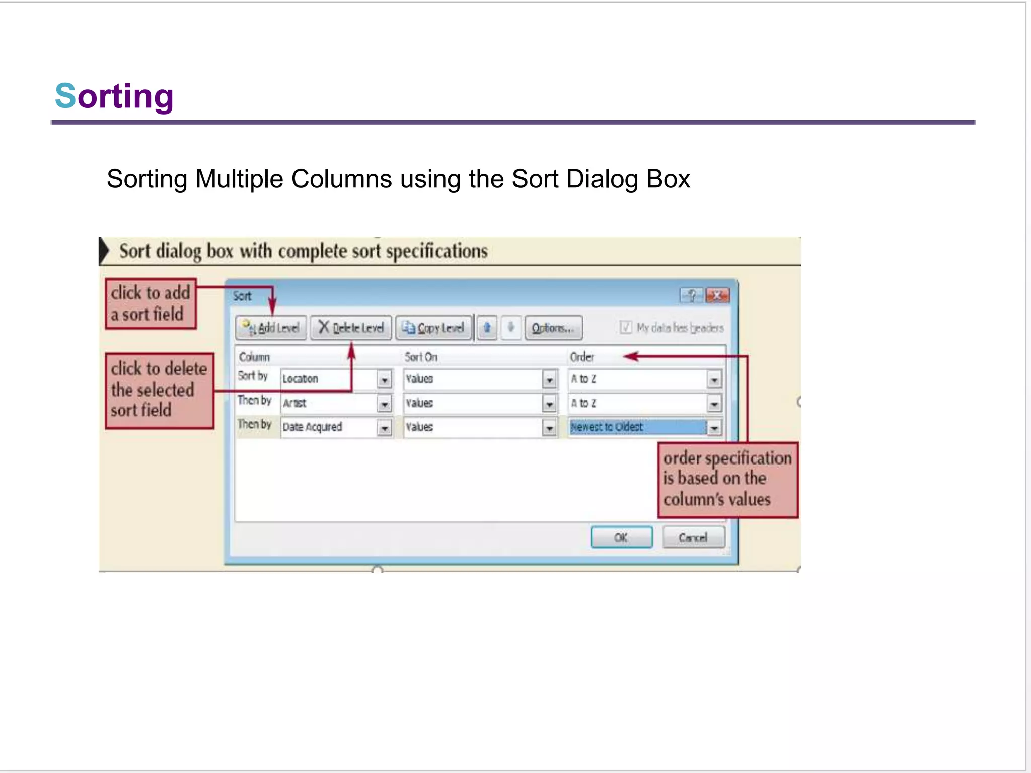
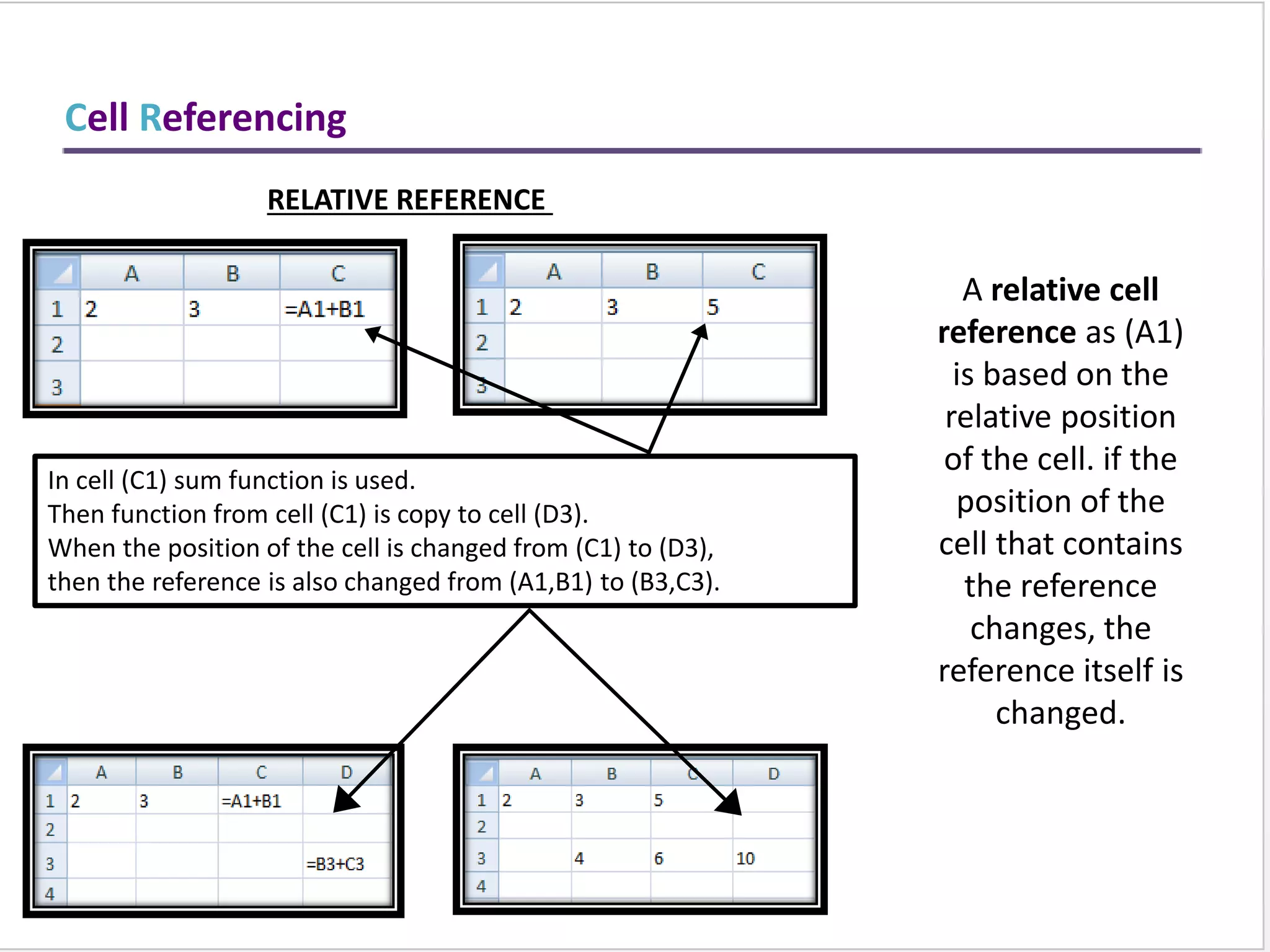
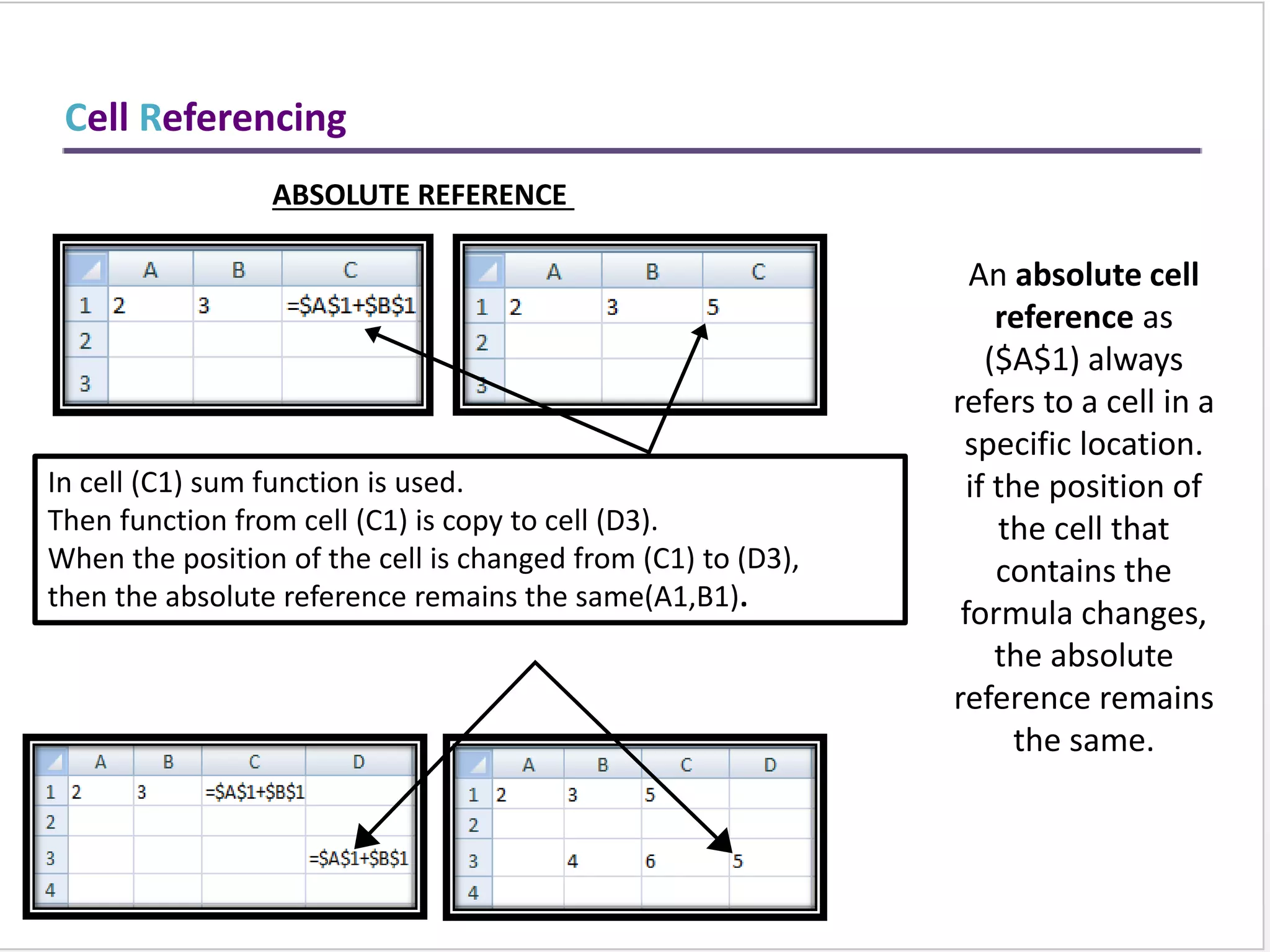
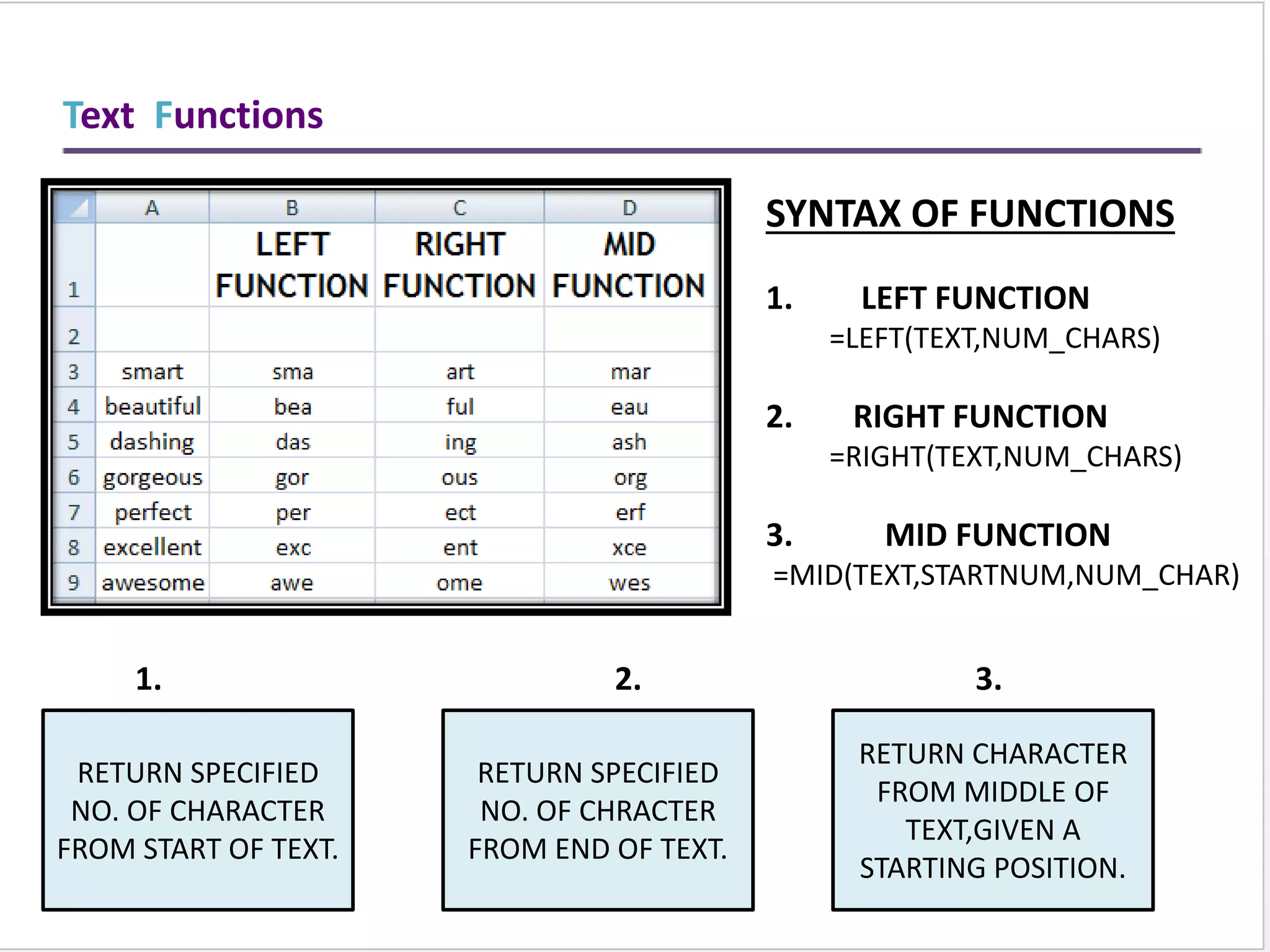
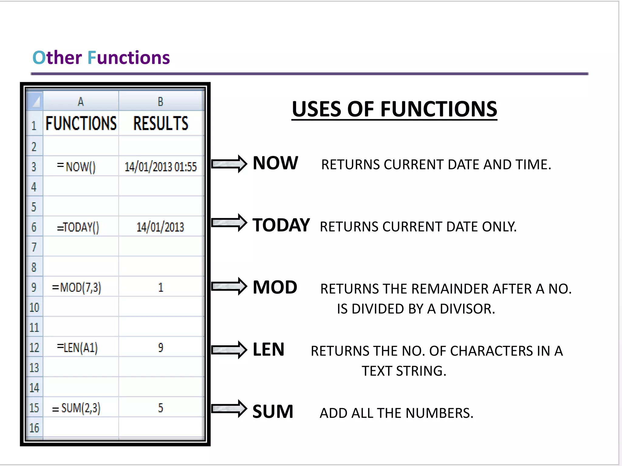
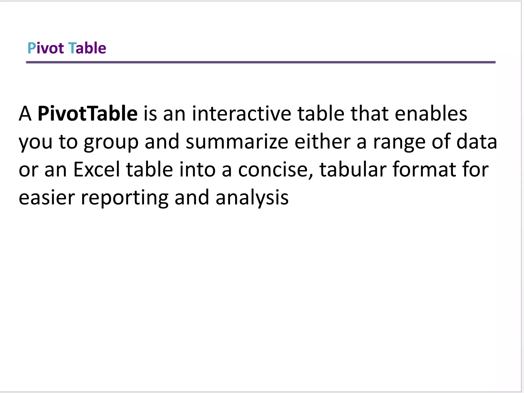
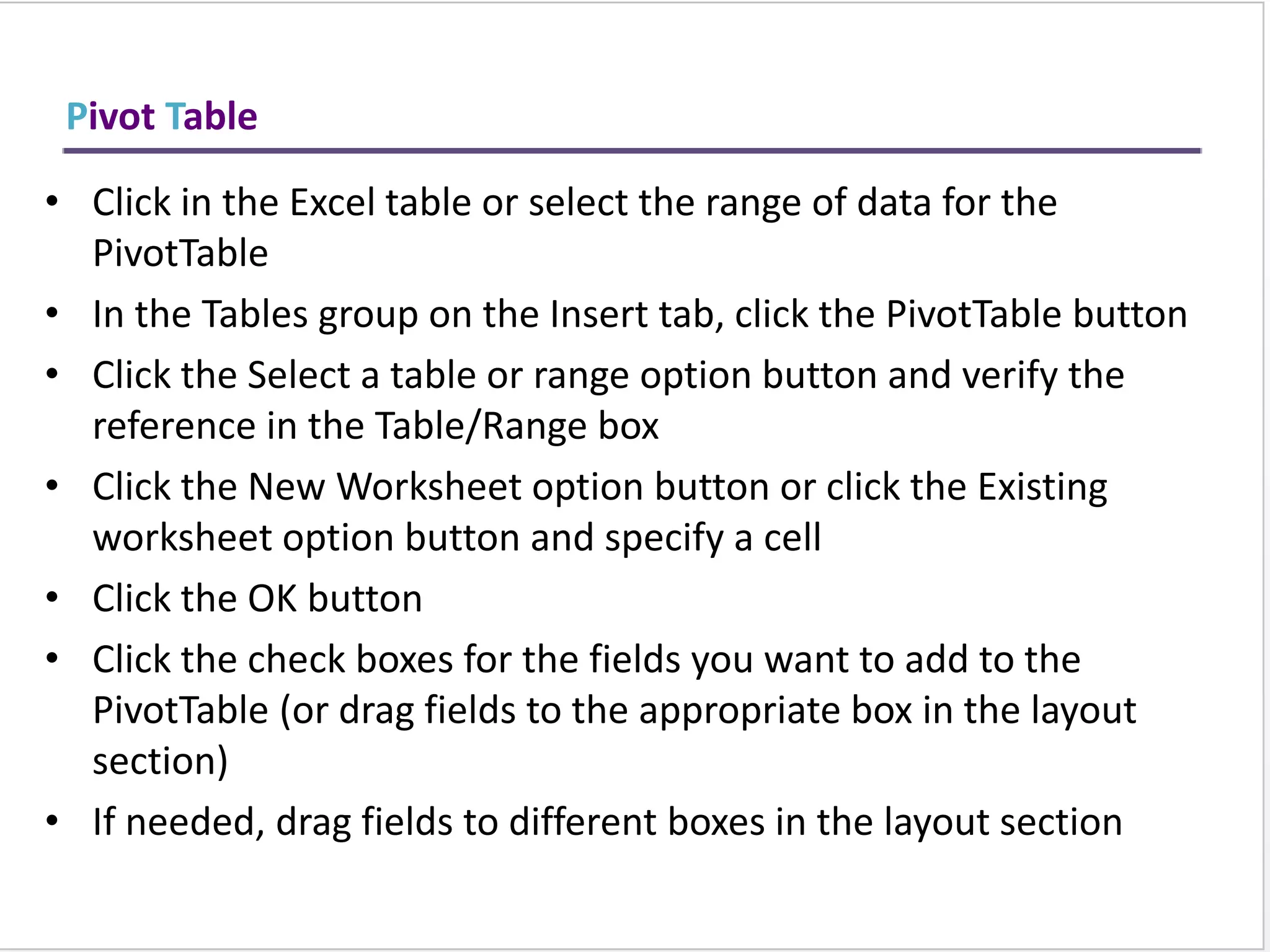
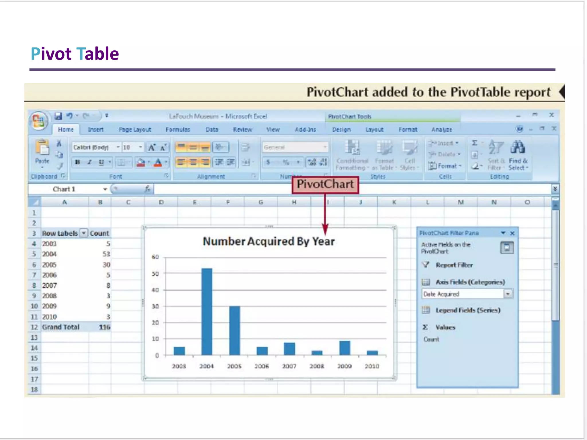
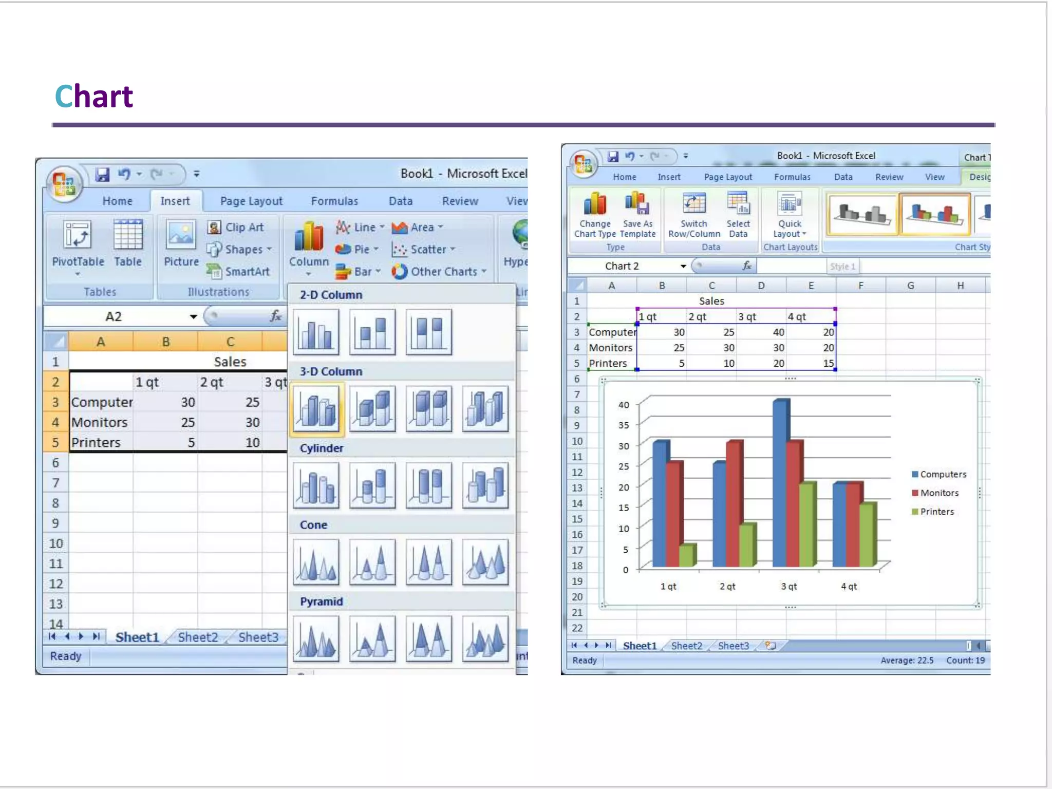
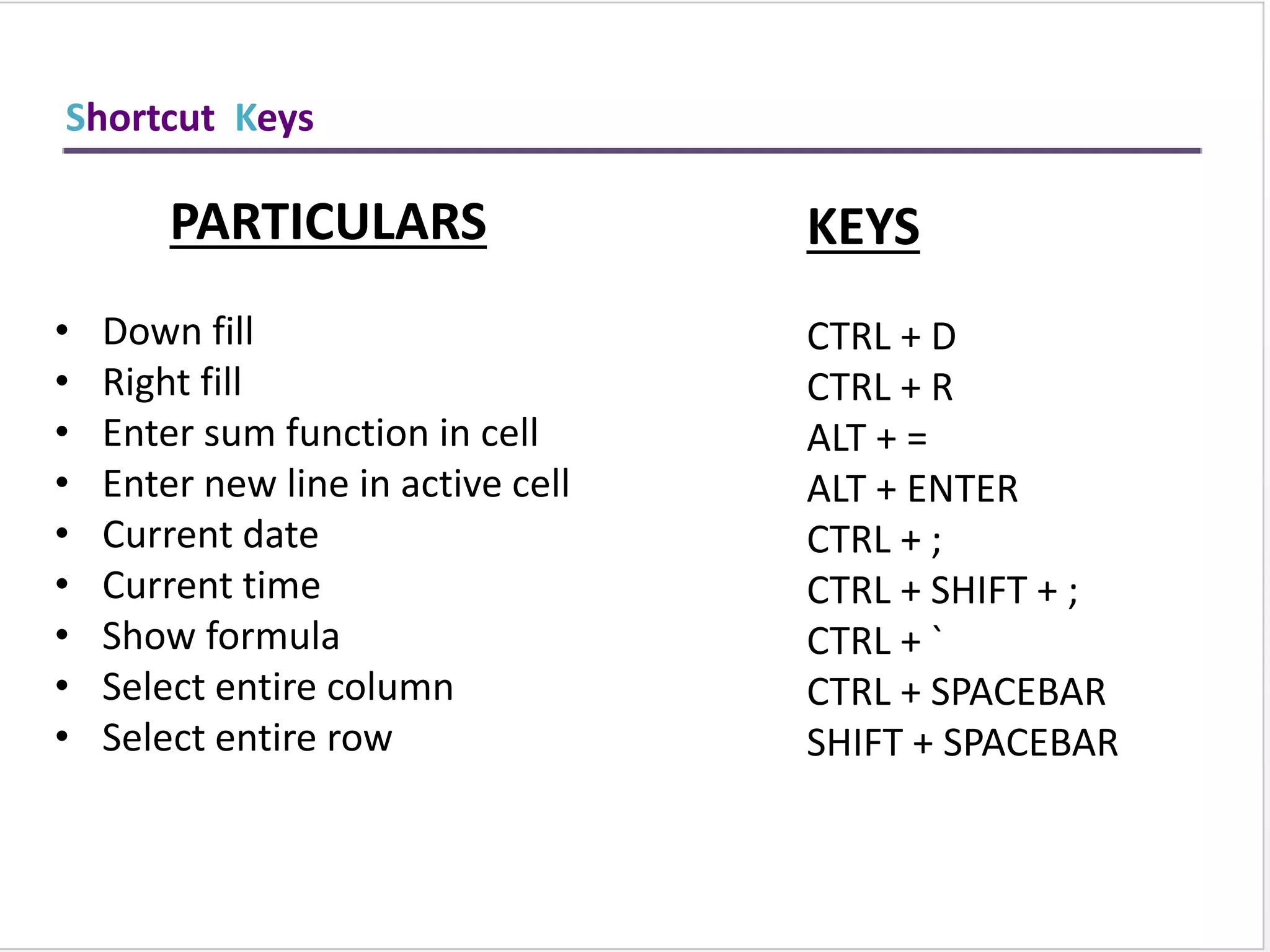
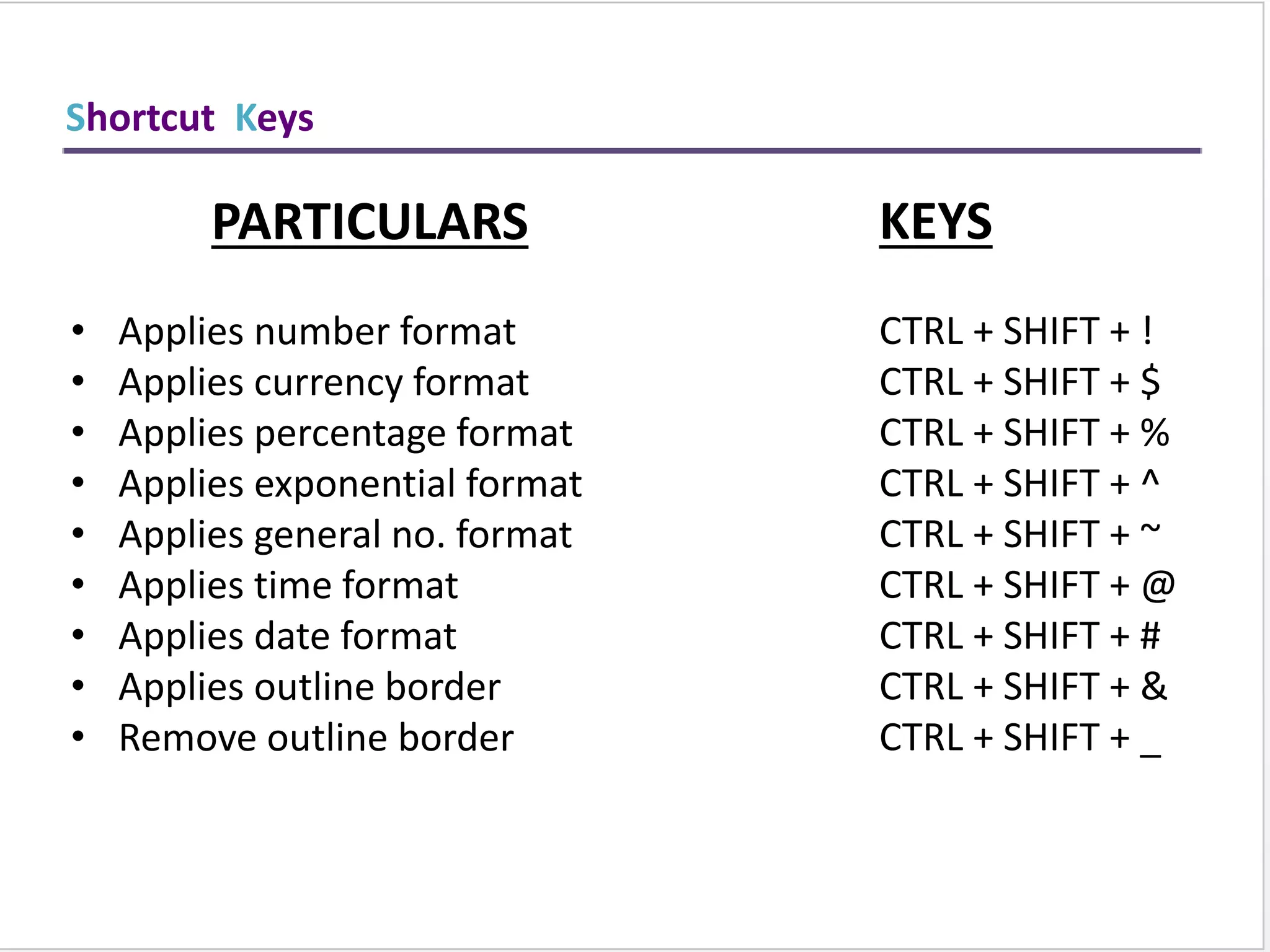
Welcome To The Training
TRAINING ON
Business Excel
Presented by:
Nahid Mohammad Ishtiaq
Objective of the Training
Contents of Training
 Introduction to Excel Office Button
 Ribbons
 Working With Cells
 Formatting Text
 Conditional Formatting
 To insert Rows & Columns
 Editing Fill
 Sorting
 Cell Referencing
 Freeze
 Functions
 PivotTable
 Chart
 Shortcut Keys
Introduction to MS-Excel
 Excel is a computer program used to create electronic
spreadsheets.
 Within excel user can organize data ,create chart and perform
calculations.
 Excel is a convenient program because it allow user to create
large spreadsheets, reference information, and it allows for
better storage of information.
 Excels operates like other Microsoft(MS) office programs and
has many of the same functions and shortcuts of other MS
programs.
Office Button Contains..
NEW-TO OPEN NEW WORKBOOK.
(CTRL+N)
OPEN-TO OPEN EXISTING DOCUMENT
(CTRL+O)
SAVE-TO SAVE A DOCUMENT.
(CTRL+S)
SAVE AS-TO SAVE COPY DOCUMENT.
(F12)
PRINT-TO PRINT A DOCUMENT.
(CTRL+P)
PREPARE-TO PREPARE DOCUMENT FOR DISTRIBUTION.
SEND-TO SEND A COPY OF DOCUMENT TO OTHER PEOPLE.
PUBLISH-TO DISTRIBUTE DOCUMENT TO OTHER PEOPLE.
CLOSE-TO CLOSE A DOCUMENT (CTRL+W).
Ribbons
TABS:THERE ARE SEVEN TABS ACROSS THE TOP OF THE
EXCEL WINDOW.
GROUPS: GROUPS ARE SETS OF RELATED
COMMANDS,DISPLAYED ON TABS.
COMMANDS: A COMMAND IS A BUTTON,A MENU OR A
BOX WHERE YOU ENTER INFORMATION.
1
2
3
TABS
GROUPS
COMMANDS
Home
Ribbon
Sizing
Button
s
Help Button
Quick Access
Toolbar
Column Letter
Headings
Row Numbers
Ribbon
Tabs
Formula Bar
Contents of
Active Cell
displayed on
Formula Bar
View Buttons Zoom
Sheet Tabs Insert Worksheet
Button
Scroll
Bars
Fx Insert
Function
Button
Name Box
Overview of Excel
Working with Cells
TO COPY AND PASTE CONTENTS:
Select the cell or cells you wish to copy.
Click the Copy command in the Clipboard group on the Home tab.
Select the cell or cells where you want to paste the information.
Click the Paste command.
The copied information will now appear in the new cells.
To Cut and Paste Cell Contents:
Select the cell or cells you wish to cut.
Click the Cut command in the Clipboard group on the Home tab.
Select the cell or cells where you want to paste the information.
Click the Paste command.
The cut information will be removed and now appear in the new cells.
Working with Cells
Formatting Text
TO FORMAT TEXT IN BOLD,
ITALICS OR UNDERLINE:
Left-click a cell to select it or drag your
cursor over the text in the formula bar to
select it.
Click the Bold, Italics or underline
command.
TO CHANGE THE FONT STYLE:
Select the cell or cells you want to format.
Left-click the drop-down arrow next to the
Font Style box on the Home tab.
Select a font style from the list.
TO CHANGE THE FONT SIZE:
Select the cell or cells you want to format.
Left-click the drop-down arrow next to the
Font Size box on the Home tab.
Select a font size from the list.
TO ADD A BORDER:
Select the cell or cells you want to format.
Click the drop-down arrow next to the
Borders command on the Home tab. A
menu will appear with border options.
Formatting Text
TO CHANGE THE TEXT COLOUR:
Select the cell or cells you want to format.
Left-click the drop-down arrow next to the Text
Color command. A color palette will appear.
Select a color from the palette.
TO ADD A FILL COLOUR:
Select the cell or cells you want to
format.
Click the Fill command. A color palette
will appear.
Select a color from the palette.
Formatting Text
Conditional Formatting
TO APPLY CONDITIONAL FORMATTING:
Select the cells you would like to format.
Select the Home tab.
Locate the Styles group.
Click the Conditional Formatting command. A menu will
appear with your formatting options.
TO REMOVE CONDITIONAL FORMATTING:
Click the Conditional Formatting command.
Select Clear Rules.
Choose to clear rules from the entire worksheet or the selected
cells.
TO MANAGE CONDITIONAL FORMATTING:
Click the Conditional Formatting command.
Select Manage Rules from the menu. The
Conditional Formatting Rules Manager dialog box
will appear. From here you can edit a rule, delete a
rule, or change the order of rules.
TO APPLY NEW FORMATTING:
Click the Conditional Formatting
command. Select New Rules from the
menu. There are different rules, you
can apply these rules to differentiate
particular cell.
Conditional Formatting
To Insert Rows & Coloums
TO INSERT ROWS:
Select the row below where you want the new row to appear.
Click the Insert command in the Cells group on the Home tab. The row will appear.
To Insert Columns:
Select the column to the right of where you want the column to appear.
Click the Insert command in the Cells group on the Home tab. The column will
appear.
NOTE:
1. The new row always
appears above the selected
row.
2. The new column always
appears to the left of the
selected column.
Editing - Fill
 IN THE LOWER RIGHT HAND CORNER OF THE ACTIVE CELL IS
EXCEL’S “FILL HANDLE”.WHEN YOU HOLD YOUR MOUSE
OVER THE TOP OF IT, YOUR CURSOR WILL TURN TO A
CROSSHAIR.
 IF YOU HAVE JUST ONE CELL SELECTED, IF YOU CLICK AND
DRAG TO FILL DOWN A COLUMN OR ACROSS A ROW, IT
WILL COPY THAT NUMBER OR TEXT TO EACH OF THE OTHER
CELLS.
 IF YOU HAVE TWO CELLS SELECTED, EXCEL WILL FILL IN A
SERIES. IT WILL COMPLETE THE PATTERN.FOR EXAMPLE,IF
YOU PUT 4 AND 8 IN TWO CELLS SELECT THEM,CLICK AND
DRAG THE FILL HANDLE ,EXCEL WILL CONTINUE THE
PATTERN WITH 12,16,20.ETC.
 EXCEL CAN ALSO AUTO- FILL SERIES OF DATES, TIMES, DAYS
OF THE WEEK, MONTHS.
Sorting
TO SORT IN ALPHABETICAL ORDER:
Select a cell in the column you want to sort (In
this example, we choose a cell in column Q).
Click the Sort & Filter command in the Editing
group on the Home tab.
Select Sort A to Z. Now the information in the
Category column is organized in alphabetical
order.
TO SORT FROM SMALLEST TO LARGEST:
Select a cell in the column you want to sort (In
this example, we choose a cell in column Q).
Click the Sort & Filter command in the Editing
group on the Home tab.
Select From Smallest to Largest. Now the
information is organized from the smallest to
largest amount.
Sorting
Sorting Multiple Columns using the Sort Dialog Box
Cell Referencing
A relative cell
reference as (A1)
is based on the
relative position
of the cell. if the
position of the
cell that contains
the reference
changes, the
reference itself is
changed.
In cell (C1) sum function is used.
Then function from cell (C1) is copy to cell (D3).
When the position of the cell is changed from (C1) to (D3),
then the reference is also changed from (A1,B1) to (B3,C3).
RELATIVE REFERENCE
Cell Referencing
An absolute cell
reference as
($A$1) always
refers to a cell in a
specific location.
if the position of
the cell that
contains the
formula changes,
the absolute
reference remains
the same.
In cell (C1) sum function is used.
Then function from cell (C1) is copy to cell (D3).
When the position of the cell is changed from (C1) to (D3),
then the absolute reference remains the same(A1,B1).
ABSOLUTE REFERENCE
Cell Referencing
In cell (C1) sum function is used.
Then function from cell (C1) is copy to cell (D3).
When the position of the cell is changed from (C1) to (D3),
then row reference is changed(from 1 to 3) but column
reference remains same(A,B).
A mixed reference
has either an
absolute column
and relative row or
absolute row and
relative column. an
absolute column
reference takes the
form $A1, $B1.an
absolute row
reference takes the
form B$1, B$1.
MIXED REFERENCE
Freeze
• Freezing a row or column lets you keep headings visible
as you work with the data in a large worksheet
• To freeze a row or column, you select the cell
immediately below the row(s) and to the right of the
column(s) you want to freeze
• Click the View tab on the Ribbon
• In the Window group, click the Freeze Panes button
Freeze
Logical Functions
=
=
=
=
=
=
SYNTAX OF DATEDIF
=DATEDIF(START_DATE,END_DATE,”INTERVAL”)
START DATE-
Date from which u want to
calculate difference.
END DATE-
Date up to which u want to
calculate difference.
INTERVAL-
Form in which u want to calculate
difference.
This says that I
am 19 years 6
months & 18
days old
“ D ” - D AY S
“ M ” - M O N T H S
“ Y ” - Y E A RS
“ Y M ” - M O N T H S OV E R Y E A R
“ M D ” - D AY S OV E R M O N T H
SYNTAX OF SUMIF
=SUMIF(RANGE,CRITERIA,SUM_RANGE)
RANGE-
Range of cells on which conditions are
applied.
CRITERIA-
Condition that defines which cell or
cells will be added.
SUM RANGE-
Actual cells to sum.
NOTE:-
If sum range is not used then range is
used for sum.
WITHOUT
SUM_RANGE
Logical Functions
SYNTAX OF IF
=IF(LOGICAL TEXT, VALUE IF TRUE, VALUE IF FALSE)
LOGICAL TEXT-
Any value or expression that can be
evaluated to TRUE or FALSE.
VALUE IF TRUE-
Value that is returned if logical text is
TRUE.
VALUE IF FALSE-
Value that is returned if logical text is
FALSE.
IN COLUMN B DIFFERENT CONDITIONS ARE USED AND BASED
ON THIS, IN COLUMN C DIFFERENT RESULTS ARE SHOWN.
=
=
=
=
=
=
=
Logical Functions
Count Functions
SYNTAX OF FUNCTIONS
1. COUNT
=COUNT(VALUE1,VALUE2,…)
2. COUNTA
=COUNTA(VALUE1,VALUE2,…)
3. COUNTBLANK
=COUNTBLANK(RANGE)
4. COUNTIF
=COUNTIF(RANGE,CRITERIA)
COUNT ONLY
CELLS THAT
CONTAINS
NUMBER.
COUNT CELLS
THAT ARE NOT
EMPTY.
COUNT CELLS
THAT ARE
BLANK.
COUNT NO. OF
CELLS THAT MEET
GIVEN
CONDITION.
1. 2. 3. 4.
COUNT ONLY
CELLS THAT
CONTAINS
NUMBER.
COUNT CELLS
THAT ARE NOT
EMPTY.
COUNT CELLS
THAT ARE
BLANK.
COUNT NO. OF
CELLS THAT MEET
GIVEN
CONDITION.
Text Functions
SYNTAX OF FUNCTIONS
1. LOWER FUNCTION
=LOWER(TEXT)
2. UPPER FUNCTION
=UPPER(TEXT)
3. PROPER FUNCTION
=PROPER(TEXT)
TO CONVERT TEXT
FROM CAPITAL TO
SMALL.
TO CAPITALISED EACH
WORD OF TEXT.
TO CONVERT TEXT
FROM SMALL TO
CAPITAL.
1. 2. 3.
Text Functions
SYNTAX OF FUNCTIONS
1. LEFT FUNCTION
=LEFT(TEXT,NUM_CHARS)
2. RIGHT FUNCTION
=RIGHT(TEXT,NUM_CHARS)
3. MID FUNCTION
=MID(TEXT,STARTNUM,NUM_CHAR)
RETURN SPECIFIED
NO. OF CHARACTER
FROM START OF TEXT.
RETURN SPECIFIED
NO. OF CHRACTER
FROM END OF TEXT.
RETURN CHARACTER
FROM MIDDLE OF
TEXT,GIVEN A
STARTING POSITION.
1. 2. 3.
Other Functions
=
=
NOW RETURNS CURRENT DATE AND TIME.
TODAY RETURNS CURRENT DATE ONLY.
MOD RETURNS THE REMAINDER AFTER A NO.
IS DIVIDED BY A DIVISOR.
LEN RETURNS THE NO. OF CHARACTERS IN A
TEXT STRING.
SUM ADD ALL THE NUMBERS.
USES OF FUNCTIONS
=
=
=
Pivot Table
A PivotTable is an interactive table that enables
you to group and summarize either a range of data
or an Excel table into a concise, tabular format for
easier reporting and analysis
• Click in the Excel table or select the range of data for the
PivotTable
• In the Tables group on the Insert tab, click the PivotTable button
• Click the Select a table or range option button and verify the
reference in the Table/Range box
• Click the New Worksheet option button or click the Existing
worksheet option button and specify a cell
• Click the OK button
• Click the check boxes for the fields you want to add to the
PivotTable (or drag fields to the appropriate box in the layout
section)
• If needed, drag fields to different boxes in the layout section
Pivot Table
Pivot Table
Pivot Table
Pivot Table
Summarize Values
Pivot Table
Pivot Table
Chart
Chart
Shortcut Keys
PARTICULARS
• Edit the active cell
• Create a chart
• Insert cell comment
• Function dialogue box
• Insert a new worksheet
• Name manager dialogue box
• Visual basic editor
• Macro dialogue box
• Hide the selected columns
• Unhide the columns
• Hide the selected rows
• Unhide the rows
• Select all cells with comment
KEYS
F2
F11
SHIFT + F2
SHIFT + F3
SHIFT + F11
CTRL + F3
ALT + F11
ALT + F8
CTRL + 0
CTRL + SHIFT + 0
CTRL + 9
CTRL + SHIFT + 9
CTRL + SHIFT + O
Shortcut Keys
PARTICULARS
• Down fill
• Right fill
• Enter sum function in cell
• Enter new line in active cell
• Current date
• Current time
• Show formula
• Select entire column
• Select entire row
KEYS
CTRL + D
CTRL + R
ALT + =
ALT + ENTER
CTRL + ;
CTRL + SHIFT + ;
CTRL + `
CTRL + SPACEBAR
SHIFT + SPACEBAR
Shortcut Keys
PARTICULARS
• Applies number format
• Applies currency format
• Applies percentage format
• Applies exponential format
• Applies general no. format
• Applies time format
• Applies date format
• Applies outline border
• Remove outline border
KEYS
CTRL + SHIFT + !
CTRL + SHIFT + $
CTRL + SHIFT + %
CTRL + SHIFT + ^
CTRL + SHIFT + ~
CTRL + SHIFT + @
CTRL + SHIFT + #
CTRL + SHIFT + &
CTRL + SHIFT + _
I remain
Nahid Mohammad Ishtiaq
Any Question
??????
Any Question
In order to succeed I must first believe that we can.
We wish and pray that you always succeed in whatever you do.
Conclusion
Thank You

Excellence with excel

  • 1.
    Welcome To TheTraining TRAINING ON Business Excel Presented by: Nahid Mohammad Ishtiaq
  • 2.
  • 4.
    Contents of Training Introduction to Excel Office Button  Ribbons  Working With Cells  Formatting Text  Conditional Formatting  To insert Rows & Columns  Editing Fill  Sorting  Cell Referencing  Freeze  Functions  PivotTable  Chart  Shortcut Keys
  • 5.
    Introduction to MS-Excel Excel is a computer program used to create electronic spreadsheets.  Within excel user can organize data ,create chart and perform calculations.  Excel is a convenient program because it allow user to create large spreadsheets, reference information, and it allows for better storage of information.  Excels operates like other Microsoft(MS) office programs and has many of the same functions and shortcuts of other MS programs.
  • 6.
    Office Button Contains.. NEW-TOOPEN NEW WORKBOOK. (CTRL+N) OPEN-TO OPEN EXISTING DOCUMENT (CTRL+O) SAVE-TO SAVE A DOCUMENT. (CTRL+S) SAVE AS-TO SAVE COPY DOCUMENT. (F12) PRINT-TO PRINT A DOCUMENT. (CTRL+P) PREPARE-TO PREPARE DOCUMENT FOR DISTRIBUTION. SEND-TO SEND A COPY OF DOCUMENT TO OTHER PEOPLE. PUBLISH-TO DISTRIBUTE DOCUMENT TO OTHER PEOPLE. CLOSE-TO CLOSE A DOCUMENT (CTRL+W).
  • 7.
    Ribbons TABS:THERE ARE SEVENTABS ACROSS THE TOP OF THE EXCEL WINDOW. GROUPS: GROUPS ARE SETS OF RELATED COMMANDS,DISPLAYED ON TABS. COMMANDS: A COMMAND IS A BUTTON,A MENU OR A BOX WHERE YOU ENTER INFORMATION. 1 2 3 TABS GROUPS COMMANDS
  • 8.
    Home Ribbon Sizing Button s Help Button Quick Access Toolbar ColumnLetter Headings Row Numbers Ribbon Tabs Formula Bar Contents of Active Cell displayed on Formula Bar View Buttons Zoom Sheet Tabs Insert Worksheet Button Scroll Bars Fx Insert Function Button Name Box Overview of Excel
  • 9.
    Working with Cells TOCOPY AND PASTE CONTENTS: Select the cell or cells you wish to copy. Click the Copy command in the Clipboard group on the Home tab. Select the cell or cells where you want to paste the information. Click the Paste command. The copied information will now appear in the new cells.
  • 10.
    To Cut andPaste Cell Contents: Select the cell or cells you wish to cut. Click the Cut command in the Clipboard group on the Home tab. Select the cell or cells where you want to paste the information. Click the Paste command. The cut information will be removed and now appear in the new cells. Working with Cells
  • 11.
    Formatting Text TO FORMATTEXT IN BOLD, ITALICS OR UNDERLINE: Left-click a cell to select it or drag your cursor over the text in the formula bar to select it. Click the Bold, Italics or underline command. TO CHANGE THE FONT STYLE: Select the cell or cells you want to format. Left-click the drop-down arrow next to the Font Style box on the Home tab. Select a font style from the list.
  • 12.
    TO CHANGE THEFONT SIZE: Select the cell or cells you want to format. Left-click the drop-down arrow next to the Font Size box on the Home tab. Select a font size from the list. TO ADD A BORDER: Select the cell or cells you want to format. Click the drop-down arrow next to the Borders command on the Home tab. A menu will appear with border options. Formatting Text
  • 13.
    TO CHANGE THETEXT COLOUR: Select the cell or cells you want to format. Left-click the drop-down arrow next to the Text Color command. A color palette will appear. Select a color from the palette. TO ADD A FILL COLOUR: Select the cell or cells you want to format. Click the Fill command. A color palette will appear. Select a color from the palette. Formatting Text
  • 14.
    Conditional Formatting TO APPLYCONDITIONAL FORMATTING: Select the cells you would like to format. Select the Home tab. Locate the Styles group. Click the Conditional Formatting command. A menu will appear with your formatting options. TO REMOVE CONDITIONAL FORMATTING: Click the Conditional Formatting command. Select Clear Rules. Choose to clear rules from the entire worksheet or the selected cells.
  • 15.
    TO MANAGE CONDITIONALFORMATTING: Click the Conditional Formatting command. Select Manage Rules from the menu. The Conditional Formatting Rules Manager dialog box will appear. From here you can edit a rule, delete a rule, or change the order of rules. TO APPLY NEW FORMATTING: Click the Conditional Formatting command. Select New Rules from the menu. There are different rules, you can apply these rules to differentiate particular cell. Conditional Formatting
  • 16.
    To Insert Rows& Coloums TO INSERT ROWS: Select the row below where you want the new row to appear. Click the Insert command in the Cells group on the Home tab. The row will appear. To Insert Columns: Select the column to the right of where you want the column to appear. Click the Insert command in the Cells group on the Home tab. The column will appear. NOTE: 1. The new row always appears above the selected row. 2. The new column always appears to the left of the selected column.
  • 17.
    Editing - Fill IN THE LOWER RIGHT HAND CORNER OF THE ACTIVE CELL IS EXCEL’S “FILL HANDLE”.WHEN YOU HOLD YOUR MOUSE OVER THE TOP OF IT, YOUR CURSOR WILL TURN TO A CROSSHAIR.  IF YOU HAVE JUST ONE CELL SELECTED, IF YOU CLICK AND DRAG TO FILL DOWN A COLUMN OR ACROSS A ROW, IT WILL COPY THAT NUMBER OR TEXT TO EACH OF THE OTHER CELLS.  IF YOU HAVE TWO CELLS SELECTED, EXCEL WILL FILL IN A SERIES. IT WILL COMPLETE THE PATTERN.FOR EXAMPLE,IF YOU PUT 4 AND 8 IN TWO CELLS SELECT THEM,CLICK AND DRAG THE FILL HANDLE ,EXCEL WILL CONTINUE THE PATTERN WITH 12,16,20.ETC.  EXCEL CAN ALSO AUTO- FILL SERIES OF DATES, TIMES, DAYS OF THE WEEK, MONTHS.
  • 18.
    Sorting TO SORT INALPHABETICAL ORDER: Select a cell in the column you want to sort (In this example, we choose a cell in column Q). Click the Sort & Filter command in the Editing group on the Home tab. Select Sort A to Z. Now the information in the Category column is organized in alphabetical order. TO SORT FROM SMALLEST TO LARGEST: Select a cell in the column you want to sort (In this example, we choose a cell in column Q). Click the Sort & Filter command in the Editing group on the Home tab. Select From Smallest to Largest. Now the information is organized from the smallest to largest amount.
  • 19.
    Sorting Sorting Multiple Columnsusing the Sort Dialog Box
  • 20.
    Cell Referencing A relativecell reference as (A1) is based on the relative position of the cell. if the position of the cell that contains the reference changes, the reference itself is changed. In cell (C1) sum function is used. Then function from cell (C1) is copy to cell (D3). When the position of the cell is changed from (C1) to (D3), then the reference is also changed from (A1,B1) to (B3,C3). RELATIVE REFERENCE
  • 21.
    Cell Referencing An absolutecell reference as ($A$1) always refers to a cell in a specific location. if the position of the cell that contains the formula changes, the absolute reference remains the same. In cell (C1) sum function is used. Then function from cell (C1) is copy to cell (D3). When the position of the cell is changed from (C1) to (D3), then the absolute reference remains the same(A1,B1). ABSOLUTE REFERENCE
  • 22.
    Cell Referencing In cell(C1) sum function is used. Then function from cell (C1) is copy to cell (D3). When the position of the cell is changed from (C1) to (D3), then row reference is changed(from 1 to 3) but column reference remains same(A,B). A mixed reference has either an absolute column and relative row or absolute row and relative column. an absolute column reference takes the form $A1, $B1.an absolute row reference takes the form B$1, B$1. MIXED REFERENCE
  • 23.
    Freeze • Freezing arow or column lets you keep headings visible as you work with the data in a large worksheet • To freeze a row or column, you select the cell immediately below the row(s) and to the right of the column(s) you want to freeze • Click the View tab on the Ribbon • In the Window group, click the Freeze Panes button
  • 24.
  • 25.
    Logical Functions = = = = = = SYNTAX OFDATEDIF =DATEDIF(START_DATE,END_DATE,”INTERVAL”) START DATE- Date from which u want to calculate difference. END DATE- Date up to which u want to calculate difference. INTERVAL- Form in which u want to calculate difference. This says that I am 19 years 6 months & 18 days old “ D ” - D AY S “ M ” - M O N T H S “ Y ” - Y E A RS “ Y M ” - M O N T H S OV E R Y E A R “ M D ” - D AY S OV E R M O N T H
  • 26.
    SYNTAX OF SUMIF =SUMIF(RANGE,CRITERIA,SUM_RANGE) RANGE- Rangeof cells on which conditions are applied. CRITERIA- Condition that defines which cell or cells will be added. SUM RANGE- Actual cells to sum. NOTE:- If sum range is not used then range is used for sum. WITHOUT SUM_RANGE Logical Functions
  • 27.
    SYNTAX OF IF =IF(LOGICALTEXT, VALUE IF TRUE, VALUE IF FALSE) LOGICAL TEXT- Any value or expression that can be evaluated to TRUE or FALSE. VALUE IF TRUE- Value that is returned if logical text is TRUE. VALUE IF FALSE- Value that is returned if logical text is FALSE. IN COLUMN B DIFFERENT CONDITIONS ARE USED AND BASED ON THIS, IN COLUMN C DIFFERENT RESULTS ARE SHOWN. = = = = = = = Logical Functions
  • 28.
    Count Functions SYNTAX OFFUNCTIONS 1. COUNT =COUNT(VALUE1,VALUE2,…) 2. COUNTA =COUNTA(VALUE1,VALUE2,…) 3. COUNTBLANK =COUNTBLANK(RANGE) 4. COUNTIF =COUNTIF(RANGE,CRITERIA) COUNT ONLY CELLS THAT CONTAINS NUMBER. COUNT CELLS THAT ARE NOT EMPTY. COUNT CELLS THAT ARE BLANK. COUNT NO. OF CELLS THAT MEET GIVEN CONDITION. 1. 2. 3. 4. COUNT ONLY CELLS THAT CONTAINS NUMBER. COUNT CELLS THAT ARE NOT EMPTY. COUNT CELLS THAT ARE BLANK. COUNT NO. OF CELLS THAT MEET GIVEN CONDITION.
  • 29.
    Text Functions SYNTAX OFFUNCTIONS 1. LOWER FUNCTION =LOWER(TEXT) 2. UPPER FUNCTION =UPPER(TEXT) 3. PROPER FUNCTION =PROPER(TEXT) TO CONVERT TEXT FROM CAPITAL TO SMALL. TO CAPITALISED EACH WORD OF TEXT. TO CONVERT TEXT FROM SMALL TO CAPITAL. 1. 2. 3.
  • 30.
    Text Functions SYNTAX OFFUNCTIONS 1. LEFT FUNCTION =LEFT(TEXT,NUM_CHARS) 2. RIGHT FUNCTION =RIGHT(TEXT,NUM_CHARS) 3. MID FUNCTION =MID(TEXT,STARTNUM,NUM_CHAR) RETURN SPECIFIED NO. OF CHARACTER FROM START OF TEXT. RETURN SPECIFIED NO. OF CHRACTER FROM END OF TEXT. RETURN CHARACTER FROM MIDDLE OF TEXT,GIVEN A STARTING POSITION. 1. 2. 3.
  • 31.
    Other Functions = = NOW RETURNSCURRENT DATE AND TIME. TODAY RETURNS CURRENT DATE ONLY. MOD RETURNS THE REMAINDER AFTER A NO. IS DIVIDED BY A DIVISOR. LEN RETURNS THE NO. OF CHARACTERS IN A TEXT STRING. SUM ADD ALL THE NUMBERS. USES OF FUNCTIONS = = =
  • 32.
    Pivot Table A PivotTableis an interactive table that enables you to group and summarize either a range of data or an Excel table into a concise, tabular format for easier reporting and analysis
  • 33.
    • Click inthe Excel table or select the range of data for the PivotTable • In the Tables group on the Insert tab, click the PivotTable button • Click the Select a table or range option button and verify the reference in the Table/Range box • Click the New Worksheet option button or click the Existing worksheet option button and specify a cell • Click the OK button • Click the check boxes for the fields you want to add to the PivotTable (or drag fields to the appropriate box in the layout section) • If needed, drag fields to different boxes in the layout section Pivot Table
  • 34.
  • 35.
  • 36.
  • 37.
  • 38.
  • 39.
  • 40.
  • 41.
    Shortcut Keys PARTICULARS • Editthe active cell • Create a chart • Insert cell comment • Function dialogue box • Insert a new worksheet • Name manager dialogue box • Visual basic editor • Macro dialogue box • Hide the selected columns • Unhide the columns • Hide the selected rows • Unhide the rows • Select all cells with comment KEYS F2 F11 SHIFT + F2 SHIFT + F3 SHIFT + F11 CTRL + F3 ALT + F11 ALT + F8 CTRL + 0 CTRL + SHIFT + 0 CTRL + 9 CTRL + SHIFT + 9 CTRL + SHIFT + O
  • 42.
    Shortcut Keys PARTICULARS • Downfill • Right fill • Enter sum function in cell • Enter new line in active cell • Current date • Current time • Show formula • Select entire column • Select entire row KEYS CTRL + D CTRL + R ALT + = ALT + ENTER CTRL + ; CTRL + SHIFT + ; CTRL + ` CTRL + SPACEBAR SHIFT + SPACEBAR
  • 43.
    Shortcut Keys PARTICULARS • Appliesnumber format • Applies currency format • Applies percentage format • Applies exponential format • Applies general no. format • Applies time format • Applies date format • Applies outline border • Remove outline border KEYS CTRL + SHIFT + ! CTRL + SHIFT + $ CTRL + SHIFT + % CTRL + SHIFT + ^ CTRL + SHIFT + ~ CTRL + SHIFT + @ CTRL + SHIFT + # CTRL + SHIFT + & CTRL + SHIFT + _
  • 44.
    I remain Nahid MohammadIshtiaq Any Question ?????? Any Question
  • 45.
    In order tosucceed I must first believe that we can. We wish and pray that you always succeed in whatever you do. Conclusion
  • 46.