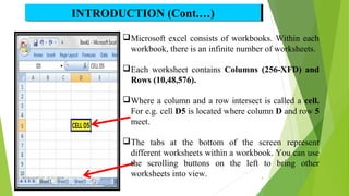
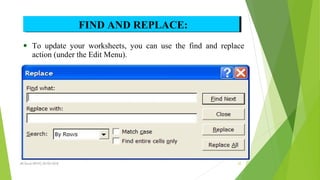
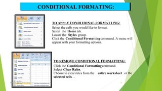
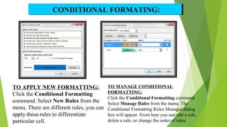
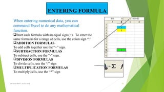
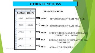
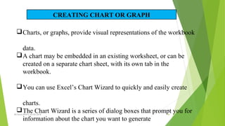
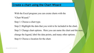
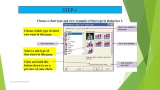
Microsoft Excel can be used to store, organize, and manipulate data. It allows data to be organized in workbooks containing worksheets with rows and columns made up of cells. Excel contains various built-in functions, formulas, charts, and data analysis tools. This document provides an overview of Excel's basic features and functions, how to enter and format data, use formulas and functions, sort and filter data, insert and delete rows/columns, and create basic charts and graphs. It demonstrates the core capabilities of Excel for organizing and analyzing data.
Excel – is the world’s most widely used spreadsheet calculating program
It is used in many places like hospitals, hotels, school and companies etc.
A program that allows you to use data to forecast, manage, predict, and present information
Lets Just Go For It! Wish you an Awesome Leaning Experience.
Subscribe to our YouTube channel: https://www.youtube.com/c/TimesRide?sub_confirmation=1
Our Official Website: http://timesride.com
Follow us:
Facebook: https://www.facebook.com/rs.agrawal.9026
Instagram: https://www.instagram.com/timesridenetwork/
Twitter: https://twitter.com/TimesRide
Pinterest: https://in.pinterest.com/ride0472/
Thank You
#AwesomeLearningExperience
#SmartQuickTips&Tricks #LeaningVideos #TimesRide #Keep Learning to Keep Winning!
MS Excel Learning for PPC Google AdWords Training CourseRanjan Jena
MS Excel learning to get expertise in Google AdWords training course. Learn all important tips and techniques in MS Excel for your fast and easy approach to Google AdWords analysis and reporting formats.
Ranjan Jena conducts Adwords Training session in Bangalore, currently with more than 45 students already graduated under his guidance and mentorship. For any training need, you can directly reach him at +91-7760969452
It is normal to be faced with so many assignments in the office set up. This demands that one is efficient with assignments. One of the skills that is very crucial, although least known is the power MS Excel This slide presents the basics of MS Excel. It attempts to give a wide overview that one needs to know about Excel. These slides presents the basic structure of Excel such as layout, functions, formulae, charts, et cetra.
Introduction to Spreadsheet, Features of Spreadsheet, Cell reference, Format cells, Data Validation, Protecting Sheets, Data Analysis in Excel: Sort, Filter, Conditional Formatting, Preparing Charts, Pivot Table, What if Analysis (Goal seek, Scenario manager), Financial Functions: NPV, PMT, PV, FV, Rate, IRR, DB, SLN, SYD. Logical Functions: IF, AND, OR, Lookup Functions: V Lookup, H Lookup, Mathematical functions and text functions
MIRCROSOFT EXCEL- brief and useful for beginners by RISHABH BANSALRishabh Bansal
the above presentation gives you a brief explanation of Microsoft excel. it includes various formulas, tips, explanations and shortcut keys that are useful for a beginner.
i found it useful, i hope u will also find it useful.
if you LIKE MY PRESENTATION you could FOLLOW ME on SLIDESHARE and FACEBOOK and add your suggestions for more.
best of luck..
Similar to Ms excel basic about Data, graph and pivot table (20)
Show drafts
volume_up
Empowering the Data Analytics Ecosystem: A Laser Focus on Value
The data analytics ecosystem thrives when every component functions at its peak, unlocking the true potential of data. Here's a laser focus on key areas for an empowered ecosystem:
1. Democratize Access, Not Data:
Granular Access Controls: Provide users with self-service tools tailored to their specific needs, preventing data overload and misuse.
Data Catalogs: Implement robust data catalogs for easy discovery and understanding of available data sources.
2. Foster Collaboration with Clear Roles:
Data Mesh Architecture: Break down data silos by creating a distributed data ownership model with clear ownership and responsibilities.
Collaborative Workspaces: Utilize interactive platforms where data scientists, analysts, and domain experts can work seamlessly together.
3. Leverage Advanced Analytics Strategically:
AI-powered Automation: Automate repetitive tasks like data cleaning and feature engineering, freeing up data talent for higher-level analysis.
Right-Tool Selection: Strategically choose the most effective advanced analytics techniques (e.g., AI, ML) based on specific business problems.
4. Prioritize Data Quality with Automation:
Automated Data Validation: Implement automated data quality checks to identify and rectify errors at the source, minimizing downstream issues.
Data Lineage Tracking: Track the flow of data throughout the ecosystem, ensuring transparency and facilitating root cause analysis for errors.
5. Cultivate a Data-Driven Mindset:
Metrics-Driven Performance Management: Align KPIs and performance metrics with data-driven insights to ensure actionable decision making.
Data Storytelling Workshops: Equip stakeholders with the skills to translate complex data findings into compelling narratives that drive action.
Benefits of a Precise Ecosystem:
Sharpened Focus: Precise access and clear roles ensure everyone works with the most relevant data, maximizing efficiency.
Actionable Insights: Strategic analytics and automated quality checks lead to more reliable and actionable data insights.
Continuous Improvement: Data-driven performance management fosters a culture of learning and continuous improvement.
Sustainable Growth: Empowered by data, organizations can make informed decisions to drive sustainable growth and innovation.
By focusing on these precise actions, organizations can create an empowered data analytics ecosystem that delivers real value by driving data-driven decisions and maximizing the return on their data investment.
Adjusting primitives for graph : SHORT REPORT / NOTESSubhajit Sahu
Graph algorithms, like PageRank Compressed Sparse Row (CSR) is an adjacency-list based graph representation that is
Multiply with different modes (map)
1. Performance of sequential execution based vs OpenMP based vector multiply.
2. Comparing various launch configs for CUDA based vector multiply.
Sum with different storage types (reduce)
1. Performance of vector element sum using float vs bfloat16 as the storage type.
Sum with different modes (reduce)
1. Performance of sequential execution based vs OpenMP based vector element sum.
2. Performance of memcpy vs in-place based CUDA based vector element sum.
3. Comparing various launch configs for CUDA based vector element sum (memcpy).
4. Comparing various launch configs for CUDA based vector element sum (in-place).
Sum with in-place strategies of CUDA mode (reduce)
1. Comparing various launch configs for CUDA based vector element sum (in-place).
Techniques to optimize the pagerank algorithm usually fall in two categories. One is to try reducing the work per iteration, and the other is to try reducing the number of iterations. These goals are often at odds with one another. Skipping computation on vertices which have already converged has the potential to save iteration time. Skipping in-identical vertices, with the same in-links, helps reduce duplicate computations and thus could help reduce iteration time. Road networks often have chains which can be short-circuited before pagerank computation to improve performance. Final ranks of chain nodes can be easily calculated. This could reduce both the iteration time, and the number of iterations. If a graph has no dangling nodes, pagerank of each strongly connected component can be computed in topological order. This could help reduce the iteration time, no. of iterations, and also enable multi-iteration concurrency in pagerank computation. The combination of all of the above methods is the STICD algorithm. [sticd] For dynamic graphs, unchanged components whose ranks are unaffected can be skipped altogether.
1. By-
Md. Alomgir Hossain
Monitoring and Evaluation Officer
World Vision Bangladesh, NJP,
Koyra, khulna, Bangladesh
MS Excel,RPATC,05/02/2018
1
2. Microsoft EXCEL is excellent for storage Data on your computer!
This presentation will cover the basic steps for the-
DATA
CHART PIOVAT
TABLE
MS Excel,RPATC,05/02/2018
2
3. Excel is an electronic spreadsheet program that can
be used for storing, organizing and manipulating
data.
It has a number of built in features and tools, such
as functions, formulas, charts, and data analysis
INTRODUCTIONINTRODUCTION
MS Excel,RPATC,05/02/2018 3
4. INTRODUCTION (Cont.…)INTRODUCTION (Cont.…)
Microsoft excel consists of workbooks. Within each
workbook, there is an infinite number of worksheets.
Each worksheet contains Columns (256-XFD) and
Rows (10,48,576).
Where a column and a row intersect is called a cell.
For e.g. cell D5 is located where column D and row 5
meet.
The tabs at the bottom of the screen represent
different worksheets within a workbook. You can use
the scrolling buttons on the left to bring other
worksheets into view.MS Excel,RPATC,05/02/2018 4
5. Features of ExcelFeatures of Excel
It allows organization, tabulation, search, and exploration of data
of large sizes.
It allows the design of professionally looking charts 3-D effects,
shadowing , transparency.
Data can be filtered and sorted.
Based on the values entered in different cells in the spreadsheet,
formulas can be defined, which automatically perform calculation.
Formatting of spreadsheet allows changing the font color, and font
style.
MS Excel,RPATC,05/02/2018 5
6. Application of ExcelApplication of Excel
To mange name list of data records.
To perform mathematical calculation easily in daily business.
Inventory management
Create forms and consolidate results
Analytical tools
Corporate budgetingMS Excel,RPATC,05/02/2018 6
8. OFFICE BUTTON CONTAINS..
NEW-TO OPEN NEW WORKBOOK.
)CTRL+N(
OPEN-TO OPEN EXISTING DOCUMENT
)CTRL+O(
SAVE-TO SAVE A DOCUMENT.
(CTRL+S)
SAVE AS-TO SAVE COPY DOCUMENT.
(F12)
PRINT-TO PRINT A DOCUMENT.
)(CTRL+P
PREPARE-TO PREPARE DOCUMENT FOR DISTRIBUTION.
SEND-TO SEND A COPY OF DOCUMENT TO OTHER PEOPLE.
PUBLISH-TO DISTRIBUTE DOCUMENT TO OTHER PEOPLE.
CLOSE-TO CLOSE A DOCUMENT (CTRL+W).
MS Excel,RPATC,05/02/2018 8
9. TABS :THERE ARE SEVEN TABS ACROSS THE TOP OFTHE EXCEL WINDOW.
GROUPS : GROUPS ARE SETS OF RELATEDCOMMANDS,DISPLAYED ON TABS
.
1
2
THE THREE PARTS
OF THE RIBBON ARE
R I B B O N S
TABS
GROUPS
COMMANDS
3 COMMANDS A BOX WHERE YOU ENTER INFORMATION:
A COMMAND IS A BUTTON,A MENU
MS Excel,RPATC,05/02/2018 9
10. Resize worksheet rows and columns
There are a number of methods for
altering row height and column width
using the mouse or menus:
Click the dividing line on the
column or row, and drag the
dividing line to change the width of
the column or height of the row
Double-click the border of a
column heading, and the column
will increase in width to match the
length of the longest entry in the
column
MS Excel,RPATC,05/02/2018 10
11. “Cell” option in the Format Menu
General Formatting.
To highlight a series of cells click and
drag the mouse over the desired area.
To move a highlighted area, click on the
border of the box and drag the box to the
desired location.
CELL FORMATCELL FORMAT
MS Excel,RPATC,05/02/2018 11
12. Change The Font Size Add a Boarder
FONT FORMATFONT FORMAT
Change The Font Color
MS Excel,RPATC,05/02/2018 12
13. 1. The new row always
appears above the
selected row.
2. The new column always
appears to the left of
the selected column.
TO INSERT ROWS:
Select the row below where you want the new row to appear.
Click the Insert command in the Cells group on the Home tab. The row will
appear.
To Insert Columns:
Select the column to the right of where you want the column to appear. Click the
Insert command in the Cells group on the Home tab. The column will appear.
INSERT/DELETE ROW/COLUMN:INSERT/DELETE ROW/COLUMN:
Note
MS Excel,RPATC,05/02/2018 13
14. You can change the view of your work
so that it is page by page.
You can insert Headers and Footers to
your work.
You can add a comments about
specific cell for future reference.
To change the order of worksheets,
click and drag the worksheet tab to the
desired order
CELL FORMAT (CONT….)CELL FORMAT (CONT….)
MS Excel,RPATC,05/02/2018 14
15. Entering Data into a Worksheet
To enter data, first make the cell in which you want to enter the data
active by clicking it.
Enter the data (text, formulas, dates, etc.) into the active cell.
Use the Alt+Enter key combination to enter text on multiple lines
within the same cell.
Use TAB key, arrow keys, or ENTER key to navigate among the
cells.
MS Excel,RPATC,05/02/2018 15
16. IN THE LOWER RIGHT HAND CORNER OF THE ACTIVE
CELL IS EXCEL’S “FILL HANDLE”.WHEN YOU HOLD
YOUR MOUSE OVER THE TOP OF IT, YOUR CURSOR
WILL TURN TO A CROSSHAIR
IF YOU HAVE JUST ONE CELL SELECTED, IF YOU
CLICK AND DRAG TO FILL DOWN A COLUMN OR
ACROSS A ROW, IT WILL COPY THAT NUMBER OR
TEXT TO EACH OF THE OTHER CELLS
IF YOU HAVE TWO CELLS SELECTED, EXCEL WILL
FILL IN A SERIES. IT WILL COMPLETE THE
PATTERN.FOR EXAMPLE,IF YOU PUT 4 AND 8 IN
TWO CELLS SELECT THEM,CLICK AND DRAG THE
FILL HANDLE ,EXCEL WILL CONTINUE THE
PATTERN WITH 12,16,20.ETC.
EXCEL CAN ALSO AUTO- FILL SERIES OF
DATES, TIMES, DAYS OF THE WEEK, MONTHS
EDDITING FILLEDDITING FILL
MS Excel,RPATC,05/02/2018 16
17. Selecting a Group of Cells
A group of selected cells is called a range.
The range is identified by its range reference, for
example, A3:C5
In an adjacent range, all cells touch each other and form
a rectangle.
To select an adjacent range, click the cell in a corner of the
range, drag the pointer to the cell in the opposite corner of
the range, and release the mouse button.
A non adjacent range includes two or more adjacent
ranges and selected cells.
To select a nonadjacent range, select the first adjacent
range or cell, press the Ctrl key as you select the other cells
or ranges you want to include, and then release the Ctrl
key and the mouse button
Range Two Types: Adjacent & Non-Adjacent
MS Excel,RPATC,05/02/2018 17
19. Select the cell or cells you wish to copy/cut.
Click the Copy command in the Clipboard group on the Home tab.
Select the cell or cells where you want to paste the information.
Click the Paste command.
The copied/cut information will now appear in the new cells
TO COPY/CUT AND PASTE CONTENTS:TO COPY/CUT AND PASTE CONTENTS:
MS Excel,RPATC,05/02/2018 19
20. TO SORT IN ALPHABETICAL ORDER:
Select a cell in the column you want to sort (In this
example, we choose a cell in column Q).
Click the Sort & Filter command in the Editing group on
the Home tab. Select Sort A to Z. Now the information in
the Category column is organized in alphabetical order.
TO SORT FROM SMALLEST TO LARGEST:
Select a cell in the column you want to sort (In this
example, we choose a cell in column Q).
Click the Sort & Filter command in the Editing group on
the Home tab. Select From Smallest to Largest. Now the
information is organized from the smallest to largest
amount.
SORTING & FILTERINGSORTING & FILTERING
MS Excel,RPATC,05/02/2018 20
21. Freezing pane
If you need the information in one column to freeze, while
still being able to scroll through the rest of the data follow
these instructions:
Step 1: Highlight a specific column.
Step 2: Go to the Window Menu and click “Freeze Panes.”
Step 3: The cells to the left of the highlighted column
should be frozen while you are still able to scroll about the
rest of the worksheet (Notice that column A remains while
column H is next to it).MS Excel,RPATC,05/02/2018 21
22. ● To update your worksheets, you can use the find and replace
action (under the Edit Menu).
FIND AND REPLACE:FIND AND REPLACE:
MS Excel,RPATC,05/02/2018 22
23. TO APPLY CONDITIONAL FORMATTING:
Select the cells you would like to format.
Select the Home tab.
Locate the Styles group.
Click the Conditional Formattingcommand. A menu will
appear with your formatting options.
TO REMOVE CONDITIONAL FORMATTING:
Click the Conditional Formattingcommand.
Select Clear Rules.
Choose to clear rules from the entire worksheet or the
selected cells .
CONDITIONAL FORMATING:CONDITIONAL FORMATING:
MS Excel,RPATC,05/02/2018 23
24. TO APPLY NEW FORMATTING:
Click the Conditional Formatting
command. Select New Rules from the
menu. There are different rules, you can
apply these rules to differentiate
particular cell.
TO MANAGE CONDITIONAL
FORMATTING:
Click the Conditional Formatting command.
Select Manage Rules from the menu. The
Conditional Formatting Rules Manager dialog
box will appear. From here you can edit a rule,
delete a rule, or change the order of rules.
CONDITIONAL FORMATING:CONDITIONAL FORMATING:
MS Excel,RPATC,05/02/2018 24
25. When entering numerical data, you can
command Excel to do any mathematical
function.
Start each formula with an equal sign (=). To enter the
same formulas for a range of cells, use the colon sign “:”
ADDITION FORMULAS
To add cells together use the “+” sign.
SUBTRACTION FORMULAS
To subtract cells, use the “-” sign.
DIVISION FORMULAS
To divide cells, use the “/” sign
MULTIPLICATION FORMULAS
To multiply cells, use the “*” sign
ENTERING FORMULA
MS Excel,RPATC,05/02/2018 25
26. A RELATIVE
CELL
REFERENCE AS
(A1) IS BASED
ON THE
RELATIVE
POSITION OF
THE CELL. IF
THE POSITION
OF THE CELL
THAT
CONTAINS THE
REFERENCE
CHANGES, THE
REFERENCE
ITSELF IS
CHANGED.
IN CELL (C1) SUM FUNCTION IS USED.
THEN FUNCTION FROM CELL (C1) IS COPY TO CELL (D3).
WHEN THE POSITION OF THE CELL IS CHANGED FROM
C1) TO (D3),THEN THE REFERENCE IS ALSO CHANGED(
FROM (A1,B1) TO (B3,C3).
CELL REFERENCINGCELL REFERENCING
MS Excel,RPATC,05/02/2018 26
27. AN ABSOLUTE
CELL
REFERENCE AS
($A$1) ALWAYS
REFERS TO A
CELL IN A
SPECIFIC
LOCATION. IF
THE POSITION
OF THE CELL
THAT CONTAINS
THE FORMULA
CHANGES, THE
ABSOLUTE
REFERENCE
REMAINS THE
SAME.
IN CELL (C1) SUM FUNCTION IS USED.
THEN FUNCTION FROM CELL (C1) IS COPY TO CELL (D3).
WHEN THE POSITION OF THE CELL IS CHANGED FROM (C1)
TO (D3),THEN THE ABSOLUTE REFERENCE REMAINS THE
SAME(A1,B1). $ IS USED FOR CONSTANT ROW OR COLUMN .
CELL REFERENCINGCELL REFERENCING
MS Excel,RPATC,05/02/2018 27
28. IN CELL (C1) SUM FUNCTION IS USED.
THEN FUNCTION FROM CELL (C1) IS COPY TO CELL (D3).
WHEN THE POSITION OF THE CELL IS CHANGED FROM
(C1) TO (D3),THEN ROW REFERENCE IS CHANGED(FROM 1
TO 3) BUT COLUMN REFERENCE REMAINS SAME(A,B).
A MIXED
REFERENCE HAS
EITHER AN
ABSOLUTE
COLUMN AND
RELATIVE ROW OR
ABSOLUTE ROW
AND RELATIVE
COLUMN. AN
ABSOLUTE
COLUMN
REFERENCE TAKES
THE FORM $A1,
$B1.AN ABSOLUTE
ROW REFERENCE
TAKES THE FORM
A$1, B$1.
CELL REFERENCINGCELL REFERENCING
MS Excel,RPATC,05/02/2018 28
29. =
=
=
=
=
=
SYNTAX OF DATEDIF
=DATEDIF(START_DATE,END_DATE,”INTERVAL”)
START DATE-
Date from which u want to
calculate difference.
END DATE-
Date up to which u want to
calculate difference.
INTERVAL-
Form in which u want to
calculate difference.
This says that I
am 19 years 6
months & 18
days old
“D” - DAYS
“M” - MONTHS
“Y” - YEARS
“YM” - MONTHS OVER YEAR
“MD” - DAYS OVER MONTH
FUNCTIONFUNCTION
MS Excel,RPATC,05/02/2018 29
30. SYNTAX OF SUMIF
=SUMIF(RANGE,CRITERIA,SUM_RANGE)
FUNCTION (CONT….)FUNCTION (CONT….)
WITHOUT
SUM_RANGE
=
=
RANGE-
Range of cells on which conditions are applied.
CRITERIA-
Condition that defines which cell or cells will be added.
SUM RANGE-
Actual cells to sum.
NOTE:-
If sum range is not used then range is used for sum.
MS Excel,RPATC,05/02/2018 30
31. SYNTAX OF IF
IF(LOGICAL TEXT, VALUE IF TRUE, VALUE IF FALSE= )
LOGICAL TEXT-
Any value or expression that can
be evaluated to TRUE or FALSE.
VALUE IF TRUE-
Value that is returned if logical
text is TRUE.
VALUE IF FALSE-
Value that is returned if logical
text is FALSE.
IN COLUMN B DIFFERENT CONDITIONS ARE USED
AND BASED ON THIS, IN COLUMN C DIFFERENT
RESULTS ARE SHOWN.
=
=
=
=
=
=
=
FUNCTIONFUNCTION
MS Excel,RPATC,05/02/2018 31
32. TEXT FUNCTIONS
SYNTAX OF FUNCTIONS
LOWER
FUNCTION=LOWER(TEXT)
UPPER
FUNCTION=UPPER(TEXT)
PROPER
FUNCTION=PROPER(TEXT)
FUNCTIONFUNCTION
MS Excel,RPATC,05/02/2018 32
34. =
=
NOW RETURNS CURRENT DATE AND TIME.
TODAY RETURNS CURRENT DATE ONLY.
MOD RETURNS THE REMAINDER AFTER A NO.
IS DIVIDED BY A DIVISOR.
LEN RETURNS THE NO. OF CHARACTERS IN A
TEXT STRING.
SUM ADD ALL THE NUMBERS.
USES OF FUNCTIONS
=
=
=
OTHER FUNCTIONSOTHER FUNCTIONS
MS Excel,RPATC,05/02/2018 34
36. CREATING CHART OR GRAPH
Charts, or graphs, provide visual representations of the workbook
data.
A chart may be embedded in an existing worksheet, or can be
created on a separate chart sheet, with its own tab in the
workbook.
You can use Excel’s Chart Wizard to quickly and easily create
charts.
The Chart Wizard is a series of dialog boxes that prompt you for
information about the chart you want to generate
MS Excel,RPATC,05/02/2018 36
37. Create a chart using the Chart Wizard
With the Excel program you can create charts with the
“Chart Wizard.”
Step 1: Choose a chart type.
Step 2: Highlight the data that you wish to be included in the chart.
Step 3: Change chart options. Here you can name the chart and the axes,
change the legend, label the data points, and many other options.
Step 4: Choose a location for the chart.
MS Excel,RPATC,05/02/2018 37
38. Choose a chart type and view examples of that type in dialog box 1.
Choose which type of chart
you want in this pane.
Select a sub-type of
that chart in this pane.
Click and hold this
button down to see a
preview of your chart.
STEP-1
MS Excel,RPATC,05/02/2018 38
39. • You can alter the data source during step 2 of the Chart Wizard and also choose
whether to organize the data source by rows or by columns.
• The data source is organized into a collection of data series.
– A data series consists of data values, which are plotted on the chart's vertical, or
Y-axis
– The data series’ category values, or X values, are on the horizontal axis, called
the X-axis
• A chart can have several data series all plotted against a common set of category
values.
Step-2:Choosing a data series
MS Excel,RPATC,05/02/2018 39
40. During the second step of the
Chart Wizard, you specify
the data to be displayed
in the chart, which is also
known as the chart's data
source.
Specify the cell range and
whether the data series is in
rows or columns.
Step-2:Choosing a data series
MS Excel,RPATC,05/02/2018 40
62. To Print a worksheet, you can use:
A menu
The Print button on the standard toolbar
The Ctrl-P keystroke to initiate a printout
of the worksheet
Excel uses the same basic methods for printing
as other Windows and Microsoft Office
applications.
PRINT A WOORKBOOK
MS Excel,RPATC,05/02/2018 62