This document provides a 3-paragraph summary of a PowerPoint presentation on Excel:
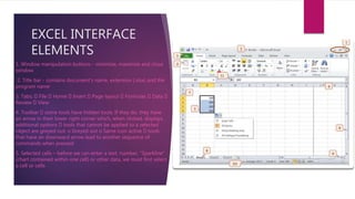
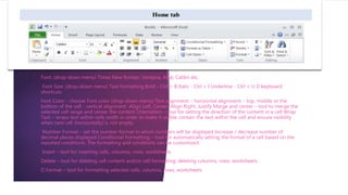
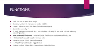
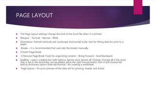
The presentation introduces Excel as a software program developed by Microsoft that allows users to organize and calculate data in a spreadsheet. It describes the basic Excel interface including worksheets, cells, formulas, and functions. Common functions like SUM, AVERAGE, MIN, and MAX are explained. The presentation also covers formatting text and numbers, inserting shapes and pictures, printing options, and other Excel features.
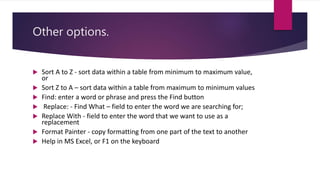
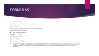
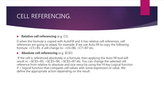
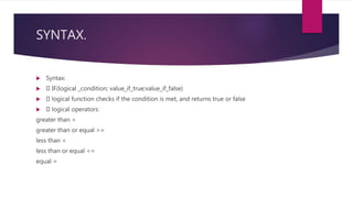
Excel functions and formulas are demonstrated including relative and absolute cell references. Logical IF functions are introduced to conditionally format cells based on comparisons. Syntax for IF functions is provided. Common Excel elements like toolbars, menus, sorting, and conditional formatting