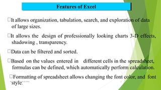
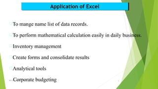
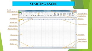
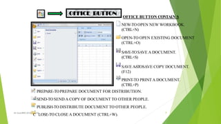
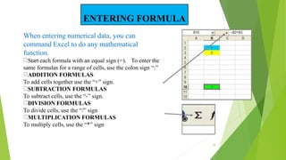
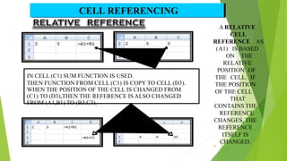
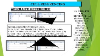
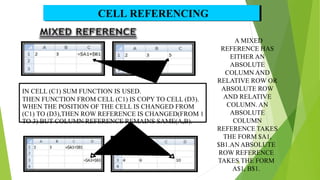
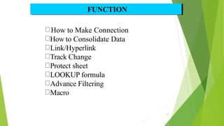
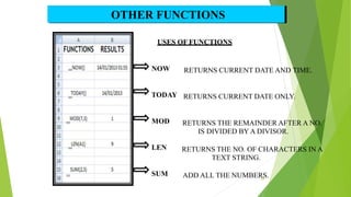
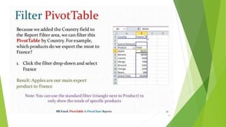
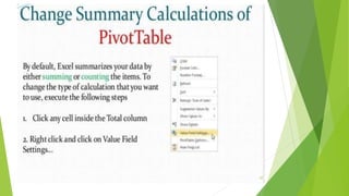
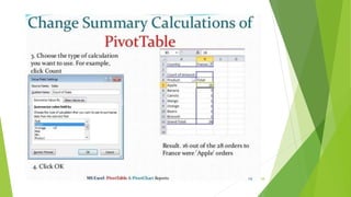
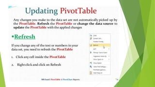
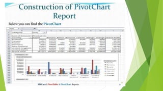
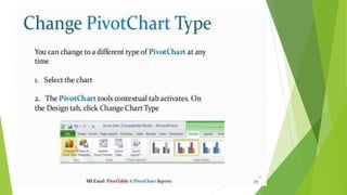
2. Course Outcomes
At the end of the course the student will be able to:
1. Solve Trigonometric, Logarithmic, Exponential, Statistical
problems and perform Matrix operations.
2. Solve civil engineering problems using VB as a tool.
3. Design structural elements by integrating excel and VB.
3. MODULE 1
Introduction to Microsoft Excel, Workbooks, Worksheets, User Interface
– navigating the interface, entering data, implicit data types, setting cell
data types, Basic operations – copy/cut, paste, paste special, row and cell
references, using cell names, Simple built-in formulae, Copying and
pasting formulae
Built-in formulae – Trigonometric, Logarithmic, Exponential, Statistical,
Matrix operations such as transpose, multiplication, inverse etc.
Plotting charts of different types, bar and pie charts, scatter plots, legend,
Using Log and Semilog scales, Customizing chart axes, Using multiple
axes, Preparing contour plots, Annotating charts.
4. Introduction to Microsoft Excel,
Microsoft Excel is a spreadsheet
developed by Microsoft for
Windows, macOS, Android and
iOS.
It features calculation, graphing
tools, pivot tables, and a macro
programming language called
Visual Basic for Applications.
5. Early History
Microsoft originally marketed a spreadsheet
program called Multiplan in 1982.
Multiplan became very popular on CP/M
systems, but on MS-DOS systems it lost
popularity to Lotus 1-2-3.
Microsoft released the first version of Excel for
the Macintosh on September 30, 1985, and the
first Windows version was 2.05 (to synchronize
with the Macintosh version 2.2) in November
1987.
Lotus was slow to bring 1-2-3 to Windows and
by the early 1990s, Excel had started to outsell 1-
2-3 and helped Microsoft achieve its position as
a leading PC software developer.
6. Microsoft EXCEL is excellent for storage Data on your computer!
This presentation will cover the basic steps for the-
DATA
CHART PIOVAT
TABLE 2
7. Excel is an electronic spreadsheet program that can
be used for storing, organizing and manipulating
data.
It has a number of built in features and tools, such
as functions, formulas, charts, and data analysis
INTRODUCTION
3
8. INTRODUCTION (Cont.…)
Microsoft excel consists of workbooks. Within each
workbook, there is an infinite number of worksheets.
Each worksheet contains Columns (256-XFD) and
Rows (10,48,576).
Where a column and a row intersect is called a cell.
For e.g. cell D5 is located where column D and row 5
meet.
The tabs at the bottom of the screen represent
different worksheets within a workbook. You can use
the scrolling buttons on the left to bring other
worksheets into view. 4
9. Features of Excel
It allows organization, tabulation, search, and exploration of data
of large sizes.
It allows the design of professionally looking charts 3-D effects,
shadowing , transparency.
Data can be filtered and sorted.
Based on the values entered in different cells in the spreadsheet,
formulas can be defined, which automatically perform calculation.
Formatting of spreadsheet allows changing the font color, and font
MS
s
Ex
t
ce
y
l,RP
l
AT
e
C,0
.
5/02/2018 5
10. Application of Excel
To mange name list of data records.
To perform mathematical calculation easily in daily business.
Inventory management
Create forms and consolidate results
Analytical tools
MS Exc
C
el,RP
o
ATC
r
,0p
5/02
o
/20
r
18ate budgeting 6
12. OFFICE BUTTON CONTAI.N.S
NEW-TO OPEN NEW WORKBOOK.
(CTRL+N)
OPEN-TO OPEN EXISTING DOCUMENT
(CTRL+O)
SA
VE-TOSAVE A DOCUMENT.
(CTRL+S)
SAVE A-STOSAVE COPY DOCUMENT.
(F12)
PRINT-TO PRINT A DOCUMENT.
(CTRL+P)
PREPARE-TOPREPARE DOCUMENT FOR DISTRIBUTION.
SEND-TO SEND A COPY OF DOCUMENT TO OTHER PEOPLE.
PUBLISH-TO DISTRIBUTE DOCUMENT TO OTHER PEOPLE.
MS Excel,RPATC,05/02/2
C
018
LOSE-TO CLOSE A DOCUMENT (CTRL+W).
8
13. TABS :THERE ARE SEVEN TABS ACROSS THE TOP OFTHE EXCEL WINDOW.
GROUPS : GROUPS ARE SETS OF RELATEDCOMMANDS,DISPLAYED ON TABS
.
1
2
THE THREE PARTS
OF THE RIBBONARE
R I B B O N S
TABS
GROUPS
COMMANDS
COMMANDS A BOX WHERE YOU ENTER INFORMATION:
A COMMAND IS A BUTTON,A MENU
9
14. Resize worksheet rows and columns
There are a number of methods for
altering row height and column width
using the mouse or menus:
Click the dividing line on the
column or row, and drag the
dividing line to change the width of
the column or height of the row
Double-click the border of a
column heading, and the column
will increase in width to match the
length of the longest entry in the
column
14
15. “Cell” option in the Format Menu
General Formatting.
To highlight a series of cells click and
drag the mouse over the desired area.
To move a highlighted area, click on the
border of the box and drag the box to the
desired location.
CELL FORMAT
15
16. Change The Font Size Add a Boarder
FONT FORMAT
Change The Font Color
12
17. INSERT/DELETE ROW/COLUMN:
Note
1. The new row always
appears above the
selected row.
2. The new column always
appears to the left of
the selected column.
TO INSERT ROWS:
Select the row below where you want the new row to appear.
Click the Insert command in the Cells group on the Home tab. The row will
appear.
To Insert Columns:
MS Ex
S
cel,
e
RP
lA
e
TC
c
,05
t/0t
2/
h
20e
18 column to the right of where you want the column to ap1
p
3 ear. Click the
Insert command in the Cells group on the Home tab. The column will appear.
18. CELL FORMAT (CONT….)
You can change the view of your work
so that it is page by page.
You can insert Headers and Footers to
your work.
You can add a comments about
specific cell for future reference.
To change the order of worksheets,
click and drag the worksheet tab to the
desired order
14
19. Entering Data into a Worksheet
To enter data, first make the cell in which you want to enter the data
active by clicking it.
Enter the data (text, formulas, dates, etc.) into the active cell.
Use the Alt+Enter key combination to enter text on multiple lines
within the same cell.
Use TAB key, arrow keys, or ENTER key to navigate among the
15
cells.
20. IN THE LOWER RIGHT HAND CORNER OF THE ACTIVE
CELL IS EXCEL’S “FILL HANDLE”.WHEN YOU HOLD
YOUR MOUSE OVER THE TOP OF IT, YOUR CURSOR
WILL TURN TO A CROSSHAIR
IF YOU HAVE JUST ONE CELL SELECTED, IF YOU
CLICK AND DRAG TO FILL DOWN A COLUMN OR
ACROSS A ROW, IT WILL COPY THAT NUMBER OR
TEXT TO EACH OF THE OTHER CELLS
IF YOU HAVE TWO CELLS SELECTED, EXCEL WILL
FILL IN A SERIES. IT WILL COMPLETE THE
PATTERN.FOR EXAMPLE,IF YOU PUT 4 AND 8 IN
TWO CELLS SELECT THEM,CLICK AND DRAG THE
FILL HANDLE ,EXCEL WILL CONTINUE THE
PATTERN WITH 12,16,20.ETC.
EXCEL CAN ALSO AUTO- FILL SERIES OF
DATES, TIMES, DAYS OF THE WEEK, MONTHS
EDDITING FILL
16
21. Selecting a Group of Cells
A group of selected cells is called a range.
The range is identified by its range reference, for
example, A3:C5
Range Two Types: Adjacent & Non-Adjacent
In an adjacent range, all cells touch each other and form
a rectangle.
To select an adjacent range, click the cell in a corner of the
range, drag the pointer to the cell in the opposite corner of
the range, and release the mouse button.
A non adjacent range includes two or more adjacent
ranges and selected cells.
To select a nonadjacent range, select the first adjacent
range or cell, press the Ctrl key as you select the other cells
or ranges you want to include, and then release the Ctrl
key and the mouse button
21
23. Select the cell or cells you wish to copy/cut.
Click the Copy command in the Clipboard group on the Home tab.
Select the cell or cells where you want to paste the information.
Click the Paste command.
The copied/cut information will now appear in the new cells
TO COPY/CUT AND PASTE CONTENTS:
23
24. TO SORT IN ALPHABETICAL ORDER:
Select a cell in the column you want to sort (In this
example, we choose a cell in column Q).
Click the Sort & Filter command in the Editing group on
the Home tab. Select Sort A to Z. Now the information in
the Category column is organized in alphabetical order.
TO SORT FROM SMALLEST TO LARGEST:
Select a cell in the column you want to sort (In this
example, we choose a cell in column Q).
Click the Sort & Filter command in the Editing group on
the Home tab. Select From Smallest to Largest. Now the
information is organized from the smallest to largest
amount.
SORTING & FILTERING
24
25. Freezing pane
If you need the information in one column to freeze, while
still being able to scroll through the rest of the data follow
these instructions:
Step 1: Highlight a specific column.
Step 2: Go to the Window Menu and click “Freeze Panes.”
Step 3: The cells to the left of the highlighted column
should be frozen while you are still able to scroll about the
rest of the worksheet (Notice that column A remains while
column H is next to it).
25
26. ● To update your worksheets, you can use the find and replace
action (under the Edit Menu).
FIND AND REPLACE:
26
27. TO APPLY CONDITIONAL FORMATTING:
Select the cells you would like to format.
Select the Hometab.
Locate the Styles group.
Click the Conditional Formatting command. A menu will
appear with your formatting options.
TO REMOVE CONDITIONAL FORMATTING:
Click the Conditional Formatting command.
Select ClearRules.
Choose to clear rules from the entire worksheet or the
selected cells .
CONDITIONAL FORMATING:
27
28. TO APPLY NEW FORMATTING:
Click the Conditional Formatting
command. Select New Rules from the
menu. There are different rules, you can
aM
p
S E
p
xce
lly
,RPAt
TC
h
,0e
5/0
s2/
e
201
r
8ules to differentiate
particular cell.
CONDITIONAL FORMATING:
TO MANAGE CONDITIONAL
FORMATTING:
Click the Conditional Formatting command.
Select Manage Rules from the menu. The
Conditional Formatting Rules Manager dialog
box will appear. From here you c
24an edit a rule,
delete a rule, or change the order of rules.
29. When entering numerical data, you can
command Excel to do any mathematical
function.
Start each formula with an equal sign (=). To enter the
same formulas for a range of cells, use the colon sign “:”
ADDITION FORMULAS
To add cells together use the “+” sign.
SUBTRACTION FORMULAS
To subtract cells, use the “-” sign.
DIVISION FORMULAS
To divide cells, use the “/” sign
MULTIPLICATION FORMULAS
To multiply cells, use the “*” sign
29
ENTERING FORMULA
30. A RELATIVE
CELL
REFERENCE AS
(A1) IS BASED
ON THE
RELATIVE
POSITION OF
THE CELL. IF
THE POSITION
OF THE CELL
THAT
CONTAINS THE
REFERENCE
CHANGES, THE
REFERENCE
ITSELF IS
CHANGED.
IN CELL (C1) SUM FUNCTION IS USED.
THEN FUNCTION FROM CELL (C1) IS COPY TO CELL (D3).
WHEN THE POSITION OF THE CELL IS CHANGED FROM
(C1) TO (D3),THEN THE REFERENCE IS ALSO CHANGED
FROM (A1,B1) TO (B3,C3).
CELL REFERENCING
30
31. AN ABSOLUTE
CELL
REFERENCE AS
($A$1) ALWAYS
REFERS TO A
CELL IN A
SPECIFIC
LOCATION. IF
THE POSITION
OF THE CELL
THAT CONTAINS
THE FORMULA
CHANGES, THE
ABSOLUTE
REFERENCE
REMAINS THE
SAME.
IN CELL (C1) SUM FUNCTION IS USED.
THEN FUNCTION FROM CELL (C1) IS COPY TO CELL (D3).
WHEN THE POSITION OF THE CELL IS CHANGED FROM (C1)
TO (D3),THEN THE ABSOLUTE REFERENCE REMAINS THE
SAME(A1,B1). $ IS USED FOR CONSTANT ROW OR COLUMN .
CELL REFERENCING
31
32. IN CELL (C1) SUM FUNCTION IS USED.
THEN FUNCTION FROM CELL (C1) IS COPY TO CELL (D3).
WHEN THE POSITION OF THE CELL IS CHANGED FROM
(C1) TO (D3),THEN ROW REFERENCE IS CHANGED(FROM 1
TO 3) BUT COLUMN REFERENCE REMAINS SAME(A,B).
CELL REFERENCING
A MIXED
REFERENCE HAS
EITHER AN
ABSOLUTE
COLUMN AND
RELATIVE ROW OR
ABSOLUTE ROW
AND RELATIVE
COLUMN. AN
ABSOLUTE
COLUMN
REFERENCE TAKES
THE FORM $A1,
$B1.AN ABSOLUTE
ROW REFERENCE
TAKES
28 THE FORM
A$1, B$1.
33. =
=
=
=
=
=
SYNTAX OF DATEDIF
=DATEDIF(START_DATE,END_DATE,”IN)TERVAL”
START DAT-E
Date from which u want to
calculate difference.
END DATE-
Date up to which u want to
calculate difference.
INTERVA-L
Form in which u want to
calculate difference.
This says that I
am 19 years 6
months & 18
days old
FUNCTION
“D” - DAYS
“M” - MONTHS
“Y” - YEARS
MS Excel,RPATC,0“
5/Y
02/2
M
018” - MONTHS OVER YEAR
“MD” - DAYS OVER MONTH
29
34. FUNCTION (CONT….)
=
=
SYNTAX OF SUMIF
=SUMIF(RANGE,CRITERIA,SUM_RANGE)
RANGE-
Range of cells on which conditions are applied.
CRITERIA-
Condition that defines which cell or cells will be added.
SUM RANGE-
Actual cells to sum.
NOTE:-
If sum range is not used then range is used for sum.
WITHOUT
SUM_RANGE
30
35. SYNTAX OF IF
=IF(LOGICAL TEXT, VALUE IF TRUE, VALUE IF FALSE)
LOGICAL TEXT-
Any value or expression that can
be evaluated to TRUE or FALSE.
VALUE IF TRUE-
Value that is returned if logical
text is TRUE.
VALUE IF FALSE-
Value that is returned if logical
text is FALSE.
IN COLUMN B DIFFERENT CONDITIONS ARE USED
AND BASED ON THIS, IN COLUMN C DIFFERENT
RESULTS ARE SHOWN.
=
=
=
=
=
=
=
FUNCTION
31
36. TEXT FUNCTIONS
SYNTAX OF FUNCTIONS
LOWER
FUNCTION=LOWER(TEXT)
UPPER
FUNCTION=UPPER(TEXT)
PROPER
FUNCTION=PROPER(TEXT)
FUNCTION
32
37. FUNCTION
37
How to Make Connection
How to Consolidate Data
Link/Hyperlink
Track Change
Protect sheet
LOOKUP formula
Advance Filtering
Macro
38. =
=
=
=
=
NOW RETURNS CURRENT DATE AND TIME.
TODAY RETURNS CURRENT DATE ONLY.
MOD RETURNS THE REMAINDER AFTER A NO.
IS DIVIDED BY A DIVISOR.
LEN RETURNS THE NO. OF CHARACTERS IN A
TEXT STRING.
SUM ADD ALL THE NUMBERS.
USES OF FUNCTIONS
OTHER FUNCTIONS
38
40. CREATING CHART OR GRAPH
information about the chart you want to generate
Charts, or graphs, provide visual representations of the workbook
data.
A chart may be embedded in an existing worksheet, or can be
created on a separate chart sheet, with its own tab in the
workbook.
You can use Excel’s Chart Wizard to quickly and easily create
charts.
The Chart Wizard is a series of dialog boxes that prompt you for
36
41. Create a chart using the Chart Wizard
41
With the Excel program you can create charts with the
“Chart Wizard.”
Step 1: Choose a chart type.
Step 2: Highlight the data that you wish to be included in the chart.
Step 3: Change chart options. Here you can name the chart and the axes,
change the legend, label the data points, and many other options.
Step 4: Choose a location for the chart.
42. Choose a chart type and view examples of that type in dialog box 1.
Choose which type of chart
you want in this pane.
Select a sub-type of
that chart in this pane.
Click and hold this
button down to see a
preview of your chart.
STEP-1
42
43. •
43
You can alter the data source during step 2 of the Chart Wizard and also choose
whether to organize the data source by rows or by columns.
The data source is organized into a collection of data series.
– A data series consists of data values, which are plotted on the chart's vertical, or
Y-axis
– The data series’ category values, or X values, are on the horizontal axis, called
the X-axis
A chart can have several data series all plotted against a common set of category
values.
•
•
Step-2:Choosing a data series
44. During the second step of the
Chart Wizard, you specify
the data to be displayed
in the chart, which is also
known as the chart's data
source.
Specify the cell range and
whether the data series is in
rows or columns.
Step-2:Choosing a data series
44
66. To Print a worksheet, you can use:
A menu
The Print button on the standard toolbar
The Ctrl-P keystroke to initiate a printout
of the worksheet
Excel uses the same basic methods for printing
as other Windows and Microsoft Office
applications.
PRINT A WOORKBOOK
66