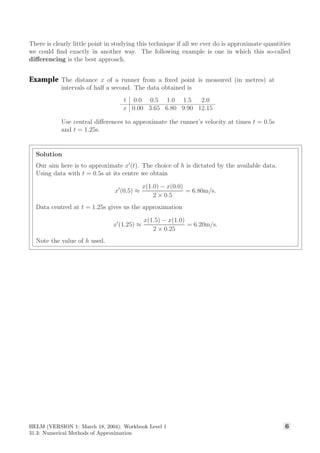
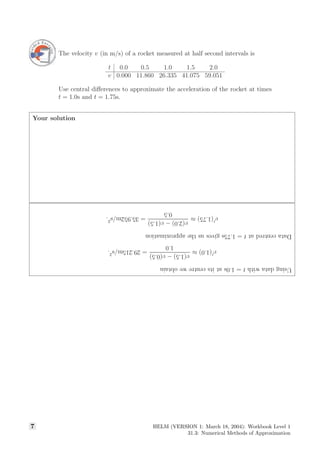
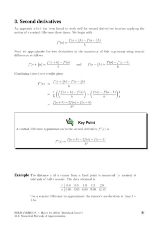
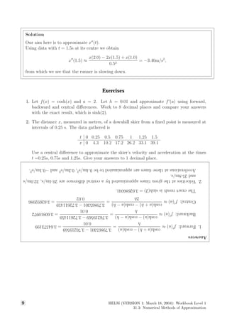
This document discusses numerical differentiation techniques to approximate the derivatives of functions, particularly focusing on first and second derivatives using forward, backward, and central difference methods. It provides step-by-step examples, including approximation calculations for specific functions like cos(x) and ln(x) at various points. The document also highlights the importance of numerical differentiation in cases where exact calculations are not feasible, using real-world data from runners and rockets to demonstrate these techniques.

1. Numerical
differentiation
31.3
Introduction
In this Section we will look at ways in which derivatives of a function may be approximated
numerically.
'
$
%
Prerequisites
Before starting this Section you should . . .
① review previous material concerning
differentiation
Learning Outcomes
After completing this Section you should be
able to . . .
✓ obtain numerical approximations to the
first and second derivatives of certain
functions

2. 1. Numerical differentiation
This Section deals with ways of numerically approximating derivatives of functions. One reason
for dealing with this now is that we will use it briefly in the next Section. But as we shall see
in these next few pages, the technique is useful in itself.
2. First derivatives
Our aim is to approximate the slope of a curve f at a particular point x = a in terms of f(a)
and the value of f at a nearby point where x = a + h. The shorter broken line in the following
diagram may be thought of as giving a decent approximation to the required slope (shown by
the longer broken line), if h is small enough.
a a+h
f
x
This slope approximates f (a)
Slope of line is f (a)
So we might approximate
f (a) ≈ slope of short broken line =
difference in the y-values
difference in the x-values
=
f(a + h) − f(a)
h
.
This is called a one-sided or forward difference approximation to the derivative of f.
A second version of this arises on considering a point to the left of a, rather than to the right
as we did above. In this case we obtain the approximation
f (a) ≈
f(a) − f(a − h)
h
This is another one-sided difference, called a backward difference, approximation to f (a).
A third method for approximating the first derivative of f can be seen in the next diagram.
HELM (VERSION 1: March 18, 2004): Workbook Level 1
31.3: Numerical Methods of Approximation
2

3. a a+h
f
This slope approximates f (a)
Slope of line is f (a)
a − h x
Here we approximate as follows
f (a) ≈ slope of short broken line =
difference in the y-values
difference in the x-values
=
f(x + h) − f(x − h)
2h
This is called a central difference approximation to f (a).
Key Point
Three approximations to the derivative f (a) are
1. the one sided (forward) difference
f(a + h) − f(a)
h
2. the one sided (backward) difference
f(a) − f(a − h)
h
3. the central difference
f(a + h) − f(a − h)
2h
In practice, the central difference formula is the most accurate.
3 HELM (VERSION 1: March 18, 2004): Workbook Level 1
31.3: Numerical Methods of Approximation

4. These first, rather artificial, examples will help fix our ideas before we move on to more realistic
applications.
Example Use a forward difference, and the values of h shown, to approximate the deriva-
tive of cos(x) at x = π/3.
(a) h = 0.1 (b) h = 0.01 (c) h = 0.001 (d) h = 0.0001
Work to 8 decimal places throughout.
Solution
(a) f (a) ≈
cos(a + h) − cos(a)
h
=
0.41104381 − 0.5
0.1
= −0.88956192
(b) f (a) ≈
cos(a + h) − cos(a)
h
=
0.49131489 − 0.5
0.01
= −0.86851095
(c) f (a) ≈
cos(a + h) − cos(a)
h
=
0.49913372 − 0.5
0.001
= −0.86627526
(d) f (a) ≈
cos(a + h) − cos(a)
h
=
0.49991339 − 0.5
0.0001
= −0.86605040
One advantage of doing a simple example first is that we can compare these approximations
with the exact value which is
f (a) = − sin(π/3) = −
√
3
2
= −0.86602540
to 8 decimal places. Notice that second to fourth approximations in the example above have
one extra accurate decimal place when compared with the previous approximation.
Example Use a central difference, and the value of h shown, to approximate the deriva-
tive of cos(x) at x = π/3.
(a) h = 0.1 (b) h = 0.01 (c) h = 0.001 (d) h = 0.0001
Work to 8 decimal places throughout.
Solution
(a) f (a) ≈
cos(a + h) − cos(a − h)
2h
=
0.41104381 − 0.58396036
0.2
= −0.86458275
(b) f (a) ≈
cos(a + h) − cos(a − h)
2h
=
0.49131489 − 0.50863511
0.02
= −0.86601097
(c) f (a) ≈
cos(a + h) − cos(a − h)
2h
=
0.49913372 − 0.50086578
0.002
= −0.86602526
(d) f (a) ≈
cos(a + h) − cos(a − h)
2h
=
0.49991339 − 0.50008660
0.0002
= −0.86602540
This time each successive approximation has two extra accurate decimal places. This pattern
continues in the following exercise.
HELM (VERSION 1: March 18, 2004): Workbook Level 1
31.3: Numerical Methods of Approximation
4

5. Let f(x) = ln(x) and a = 3. Using both a forward and a central difference, and
working to 8 decimal places, approximate f (a) using h = 0.1 and h = 0.01.
(Note that this is another example where we can work out the exact answer,
which in this case is 1
3
.)
Your solution
Usingtheforwarddifferencewefind,forh=0.1
f(a)≈
ln(a+h)−ln(a)
h
=
1.13140211−1.09861229
0.1
=0.32789823
andforh=0.01weobtain
f(a)≈
ln(a+h)−ln(a)
h
=
1.10194008−1.09861229
0.01
=0.33277901
Usingcentraldifferencesthetwoapproximationstof(a)are
f(a)≈
ln(a+h)−ln(a−h)
2h
=
1.13140211−1.06471074
0.2
=0.33345687
and
f(a)≈
ln(a+h)−ln(a−h)
2h
=
1.10194008−1.09527339
0.02
=0.33333457
5 HELM (VERSION 1: March 18, 2004): Workbook Level 1
31.3: Numerical Methods of Approximation

6. There is clearly little point in studying this technique if all we ever do is approximate quantities
we could find exactly in another way. The following example is one in which this so-called
differencing is the best approach.
Example The distance x of a runner from a fixed point is measured (in metres) at
intervals of half a second. The data obtained is
t 0.0 0.5 1.0 1.5 2.0
x 0.00 3.65 6.80 9.90 12.15
Use central differences to approximate the runner’s velocity at times t = 0.5s
and t = 1.25s.
Solution
Our aim here is to approximate x (t). The choice of h is dictated by the available data.
Using data with t = 0.5s at its centre we obtain
x (0.5) ≈
x(1.0) − x(0.0)
2 × 0.5
= 6.80m/s.
Data centred at t = 1.25s gives us the approximation
x (1.25) ≈
x(1.5) − x(1.0)
2 × 0.25
= 6.20m/s.
Note the value of h used.
HELM (VERSION 1: March 18, 2004): Workbook Level 1
31.3: Numerical Methods of Approximation
6

7. The velocity v (in m/s) of a rocket measured at half second intervals is
t 0.0 0.5 1.0 1.5 2.0
v 0.000 11.860 26.335 41.075 59.051
Use central differences to approximate the acceleration of the rocket at times
t = 1.0s and t = 1.75s.
Your solution
Usingdatawitht=1.0satitscentreweobtain
v(1.0)≈
v(1.5)−v(0.5)
1.0
=29.215m/s2
.
Datacentredatt=1.75sgivesustheapproximation
v(1.75)≈
v(2.0)−v(1.5)
0.5
=35.952m/s2
.
7 HELM (VERSION 1: March 18, 2004): Workbook Level 1
31.3: Numerical Methods of Approximation

8. 3. Second derivatives
An approach which has been found to work well for second derivatives involves applying the
notion of a central difference three times. We begin with
f (a) ≈
f (a + 1
2
h) − f (a − 1
2
h)
h
.
Next we approximate the two derivatives in the numerator of this expression using central
differences as follows:
f (a + 1
2
h) ≈
f (a + h) − f (a)
h
and f (a − 1
2
h) ≈
f (a) − f (a − h)
h
.
Combining these three results gives
f (a) ≈
f (a + 1
2
h) − f (a − 1
2
h)
h
≈
1
h
f (a + h) − f (a)
h
−
f (a) − f (a − h)
h
=
f(a + h) − 2f(a) + f(a − h)
h2
Key Point
A central difference approximation to the second derivative f (a) is
f (a) ≈
f(a + h) − 2f(a) + f(a − h)
h2
Example The distance x of a runner from a fixed point is measured (in metres) at
intervals of half a second. The data obtained is
t 0.0 0.5 1.0 1.5 2.0
x 0.00 3.65 6.80 9.90 12.15
Use a central difference to approximate the runner’s acceleration at time t =
1.5s.
HELM (VERSION 1: March 18, 2004): Workbook Level 1
31.3: Numerical Methods of Approximation
8

9. Solution
Our aim here is to approximate x (t).
Using data with t = 1.5s at its centre we obtain
x (1.5) ≈
x(2.0) − 2x(1.5) + x(1.0)
0.52
= −3.40m/s2
,
from which we see that the runner is slowing down.
Exercises
1. Let f(x) = cosh(x) and a = 2. Let h = 0.01 and approximate f (a) using forward,
backward and central differences. Work to 8 decimal places and compare your answers
with the exact result, which is sinh(2).
2. The distance x, measured in metres, of a downhill skier from a fixed point is measured at
intervals of 0.25 s. The data gathered is
t 0 0.25 0.5 0.75 1 1.25 1.5
x 0 4.3 10.2 17.2 26.2 33.1 39.1
Use a central difference to approximate the skier’s velocity and acceleration at the times
t =0.25s, 0.75s and 1.25s. Give your answers to 1 decimal place.
Answers
1.Forward:f(a)≈
cosh(a+h)−cosh(a)
h
=
3.79865301−3.76219569
0.01
=3.64573199
Backward:f(a)≈
cosh(a)−cosh(a−h)
h
=
3.76219569−3.72611459
0.01
=3.60810972
Central:f(a)≈
cosh(a+h)−cosh(a−h)
2h
=
3.79865301−3.72611459
0.02
=3.62692086
Theexactresultissinh(2)=3.62686041.
2.Velocitiesatthegiventimesapproximatedbyacentraldifferenceare20.4m/s,32.0m/s
and25.8m/s.
Accelerationsatthesetimesareapproximatedtobe0.4m/s2
,0.3m/s2
and−0.1m/s2
.
9 HELM (VERSION 1: March 18, 2004): Workbook Level 1
31.3: Numerical Methods of Approximation