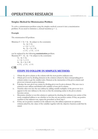
Downloaded 44 times


![OPERATIONS RESEARCH
rmakaha@facebook.com
Maclaurin Series
The infinite series expansion for f(x) about x = 0 becomes:
f '(0) is the first derivative evaluated at x = 0, f ''(0) is the second derivative evaluated at x = 0, and so
on.
[Note: Some textbooks call the series on this page Taylor Series (which they are, too), or series
expansion or power series.]
Maclaurin’s Series. A series of the form
Such a series is also referred to as the expansion (or development) of the function f(x) in powers of x, or its
expansion in the neighborhood of zero. Maclaurin’s series is best suited for finding the value of f(x) for a
value of x in the neighborhood of zero. For values of x close to zero the successive terms in the
expansion grow small rapidly and the value of f(x) can often be approximated by summing only the
first few terms.
A function can be represented by a Maclaurin series only if the function and all its derivatives exist
for x = 0. Examples of functions that cannot be represented by a Maclaurin series: 1/x, ln x, cot x.
rmmakaha@gmail.com 5](https://image.slidesharecdn.com/operationsresearch-141109234626-conversion-gate01/85/OPERATIONS-RESEARCH-5-320.jpg)


![OPERATIONS RESEARCH
Newton's method
In numerical analysis, Newton's method
after Isaac Newton and Joseph R
to the roots (or zeroes) of a real
methods, succeeded by Halley's method
(also known as the Newton–Raphson method
Raphson, is a method for finding successively better approximations
eal-valued function. The algorithm is first in the class of
method.
The Newton-Raphson method in one variable:
Given a function ƒ(x) and its derivative
is reasonably well-behaved a better approximation
ƒ '(x), we begin with a first guess x0. Provided the function
x1 is
Geometrically, x1 is the intersection point of the
process is repeated until a sufficiently accurate value is reached:
A. Description
tangent line to the graph of f, with the x
The function ƒ is shown in blue and the tangent line is in red. We see that
approximation than xn for the root
The idea of the method is as follows: one starts with an initial guess which is reasonably close to the
true root, then the function is approximated by its
tools of calculus), and one computes the
elementary algebra). This x-intercept will typically be a better approximat
than the original guess, and the method can be
Suppose ƒ : [a, b] → R is a differentiable
real numbers R. The formula for converging on the root can be easily derived. Suppose we have
some current approximation xn
referring to the diagram on the right. We know from the definition o
that it is the slope of a tangent at that point.
That is
Here, f ' denotes the derivative
rmmakaha@gmail.com
xn+1
x of the function f.
tangent line (which can be computed using the
), x-intercept of this tangent line (which is easily done with
approximation to the function's root
iterated.
function defined on the interval [a, b
. . Then we can derive the formula for a better approximation,
of the derivative at a given point
of the function f. Then by simple algebra we can derive
10
rmakaha@facebook.com
method), named
, . Householder's
x-axis. The
+is a better
h ion b] with values in the
xn+1 by
f .](https://image.slidesharecdn.com/operationsresearch-141109234626-conversion-gate01/85/OPERATIONS-RESEARCH-10-320.jpg)


![OPERATIONS RESEARCH
rmakaha@facebook.com
Conclusion:
Since all the cell values are positive the solution is optimum with the following allocations:
A Supplies 220 to 3
B Supplies 260 to 2
C Supplies 160 to 1
C Supplies 80 to 3
C Supplies 140 to 4
With a minimum cost of $ 5320.00
QUESTION
Below is a transportation problem where costs are in thousand of dollars.
SOURCES DESTINATIONS
A B C CAPACITIES
X 14 13 15 500
Y 16 15 12 400
Z 20 15 16 600
REQUIREMENTS 700 300 500
i. Solve this problem fully indicating the optimum delivery allocations and the corresponding
total delivery cost. [6 marks]
ii. There are two optimum solutions. Find the second one [4 marks].
iii. Solve the same problem considering XA is an infeasible (prohibited / impossible) route
and find the new total transportation cost [7 marks].
iv. If under consideration is a road network in a war zone, what is the simple economic effect of
bombing a bridge between X and A? [3 marks].
3 5
6
9
0
7 4
1
-4
5 12 10
rmmakaha@gmail.com 43
Solution: PART (i)
TABLEAU 1:
A B C Capacity
X 500 500
Y 200 200 400
Z 4
100 500 600
Req 700 300 500 1500
The initial solution = (500 * 14) + (200 * 16) + (15 * 200) + (100 * 15) + (500 * 16)](https://image.slidesharecdn.com/operationsresearch-141109234626-conversion-gate01/85/OPERATIONS-RESEARCH-43-320.jpg)


![OPERATIONS RESEARCH
rmakaha@facebook.com
DUMMIES:
This is an extra row or column in a transportation table with zero cost in each cell and with a
total equal to the difference between total capacity and total demand.
In an unbalance transportation problem a dummy source or destination is introduced.
12 23
43
3
10 - 51
23 0
63 33
53
51
21 -22
30 -40 0
33 1 63 13
0
0
rmmakaha@gmail.com 46
QUESTION:
The transport manager of a company has 3 factories A, B and C and four warehouses I, II, III and
IV is faced with a problem of determining the way in which factories should supply warehouses so
as to minimize the total transportation costs.
In a given month the supply requirements of each warehouse, the production capacities of the
factories and the cost of shipping one unit of product from each factory to each warehouse in $ are
shown below.
FACTORY WAREHOUSES
I II III IV PRO AVAIL
A 12 23 43 3 6
B 63 23 33 53 53
C 33 1 63 13 17
REQUIREMENTS 4 7 6 14 31
You are required to determine the minimum cost transportation plan [20 marks].
Solution:
TABLEAU 1:
I II III IV Dummy Capacity
A 4 2 6
B 5 6 14 28 53
C 17 17
Req 4 7 6 14 45 76
This is the initial solution, which costs
(4 * 12) + (2 * 23) + (5 * 23) + (6 * 33) + (14 * 53) + (28 * 0) + (17 * 0)
= $1149.00](https://image.slidesharecdn.com/operationsresearch-141109234626-conversion-gate01/85/OPERATIONS-RESEARCH-46-320.jpg)

![OPERATIONS RESEARCH
rmakaha@facebook.com
rmmakaha@gmail.com 48
Hence delivery allocations are:
Factory A Supplies Warehouse I
Factory A Supplies Warehouse IV
Factory B Supplies Warehouse II
Factory B Supplies Warehouse III
Factory B Supplies Warehouse Dummy
Factory C Supplies Warehouse II
Factory C Supplies Warehouse IV
With a minimum cost of (4 * 12) + (2 * 3) + (2 * 23) + (6 * 33) + (45 * 0) + (12 * 13) + (5 * 1)
= $459.00
QUESTION:
A well-known organization has 3 warehouse and 4 Shops. It requires transporting its goods from the
warehouse to the shops. The cost of transporting a unit item from a warehouse to a shop and the
quantity to be supplied are shown below.
DESTINATION
I II III IV TOTAL SUPPLY
SOURCE A 10 0 20 11 15
SOURCE B 12 7 9 20 25
SOURCE C 0 14 16 18 5
TOTAL DEMAND 5 15 15 10
Use any method to find the optimum transportation schedule and indicate the cost [14marks].
DEGENERATE SOLUTION:
It involves working a transportation problem if the number of used routes is equal to:
Number of rows + Number of column – 1.
However if the number of used routes can be less than the required figure we pretend that an empty
route is really used by allocating a zero quantity to that route.
MAXIMIZATION PROBLEMS:
Transportation algorithm assumes that the objective is to minimize cost. However it is possible to
use the method to solve maximization problem by either:
Multiply all the units’ contribution by – 1.
Or by subtracting each unit contribution from the maximum contribution in the
table.](https://image.slidesharecdn.com/operationsresearch-141109234626-conversion-gate01/85/OPERATIONS-RESEARCH-48-320.jpg)
![OPERATIONS RESEARCH
rmakaha@facebook.com
UNIT 3: NON-LINEAR FUNCTIONS:
HOURS: 20.
NON-LINEAR FUNCTIONS:
o MARGINAL DISTRIBUTION:
PARTIAL INTEGRATION:
Partial integration is a function with more than one variable or finding the probability of a function
with more than one variables i.e. f(X1, X2, X3, ….Xn) and is just the rate at which the values of a
function change as one of the independent variables change and all others are held constant.
Question 1:
If f(x, y) = 2(x + y –2xy) given the intervals 0= x=1, 0=y=1.
Find the marginal distribution of x = f(x).
Find the marginal distribution of y = f(x).
Solution:
Pr {0=x=1} = 0∫1 2(x + y –2xy)dx
= 2 0∫1 (x + y –2xy)dx
= 2 [x2/2 + xy + x2y]0
1
rmmakaha@gmail.com 49
= 2 [½ + y – y]
= 2[½]
= 1
Pr {0=y=1} = 0∫1 2(x + y –2xy)dy
= 2 ∫1 (x + y –2xy)dy
0= 2 [xy +y2/+ xy2]1
2 0
= 2 [x + ½ – x]
= 2[½]
= 1
Question 1:
If f(X1, X2) =(X2
1X2 + X3
1X2
2 + X1) given the intervals 0= X1=2, 1=X2 =3.
Find the marginal distribution of x = f(x).
Find the marginal distribution of y = f(x).
Find the Expected value of X1 (E(X1)).
Find the variance of X1 (Var (X1)).](https://image.slidesharecdn.com/operationsresearch-141109234626-conversion-gate01/85/OPERATIONS-RESEARCH-49-320.jpg)
![OPERATIONS RESEARCH
rmakaha@facebook.com
Solution:
Pr {0=X1=2} = 0∫2 (X2
1X2 + X3
1X2
2 + X1)dx
rmmakaha@gmail.com 50
= [X3
1X2 /3+ X4
1X2
2 /4+ X2
1/2]0
2
= [8X2 /3+ 4X2
2 + 2] – [0]
= 8X2 /3+ 4X2
2 + 2
Pr {1=X2=3} = 1∫3 (X2
1X2 + X3
1X2
2 + X1)dy
= [X2
1X2
2 /2+ X3
1X3
2 /3+ X1X2]1
3
= [9X2
1 /2+ 27X3
1 /3+ 3X2]1
3 –[X2
1 /2+ X3
2 /3+ X1]
= 9X2
1 /2+ 27X3
1 /3+ 3X2 – X2
1 /2- X3
2 /3 - X1
= 8X2
1 /2+ 26X3
1 /3+ 2X2
Expected value of E(X1) =0∫2 X. f(X1)dx
= 0∫2 X(X2
1X2 + X3
1X2
2 + X1)dx
= 0∫2 (X3
1X2 + X4
1X2
2 + X2
1)dx
= [X4
1X2 /4+ X5
1X2
2 /5+ X3
1/3]0
2
= [4X2 + 32X2
2 /5 + 8 /3] – [0]
= 4X2 + 32X2
2 /5 + 8 /3
Variance of X1 = Var (X1) = 0∫2 ([X1 - E(X1)]2 . f(X1)dx
= 0∫2 ([X1 - 4X2 + 32X2
2 /5 + 8 /3]2 * (X2
1X2 + X3
1X2
2 + X1)dx.
Question 2:
A manufacturing company produces two products bicycles and roller skates. Its fixed costs
production is: $1200 per week. Its variables costs of production are: $40 for each bicycle produced
and $15 for each pair of roller skates. Its total weekly costs in producing x bicycles and y pairs of
roller skates are therefore c= cost.
C(x, y) = 1200 + 40x + 15y for example; in producing x = 20 bicycles and y = 30 pairs of roller
skates/ week.
The manufacture experiences total cost of:
C(20, 30) = 1200 + 40(20) + 15(30)
= 1200 + 800 + 450
= 2450.
Question 3:
A manufacturing of Automobile tyres produces 3 different types: regular, green and blue tyres. If the
regular tyres sell for $60 each, the green tyres for $50 each and the blue tyres for $100 each. Find a
function giving the manufacture’s total receipts or revenue from the of x regular tyres and y green
tyres and z blue tyres.
R(x, y, z) = 60x + 50y +100z.](https://image.slidesharecdn.com/operationsresearch-141109234626-conversion-gate01/85/OPERATIONS-RESEARCH-50-320.jpg)


![OPERATIONS RESEARCH
rmakaha@facebook.com
Question 1:
Given f(X1, X2, X3) =(X1 + 2X3 + X2X3 – X2
1 - X2
2 - X2
3)
Find the gradient vector for X0 i.e. Ñf (X0) = 0.
Solution:
The necessary condition (gradient vector) Ñf (X0) = 0 is given by:
rmmakaha@gmail.com 53
df / dx1 = 1 - 2X1 = 0.
1 - 2X1 = 0. [1]
df / dx2 = X3 - 2X2 = 0.
X3 - 2X2 = 0. [2]
df / dx3 = 2 + X2 - 2X3 = 0.
2 + X2 - 2X3 = 0. [3]
(a) Finding X1 is given by 1 = 2X1
X1 = ½
(b) Equation 2 is given by X3 - 2X2 = 0.
X3 = 2X2.
(c) On equation 3 where therefore substitute X3 with 2X2.
Thus 2 + X2 - 2X3 = 0.
2 + X2 – 2(2X2) = 0.
2 + X2 – 4X2 = 0.
2 – 3X2 = 0.
X2 = 2/3.
Therefore X3 = 2X2.
X3 = 2(2 / 3)
X3 = 4/3.
Therefore X0 = (½, 2/3, 4/3)](https://image.slidesharecdn.com/operationsresearch-141109234626-conversion-gate01/85/OPERATIONS-RESEARCH-53-320.jpg)


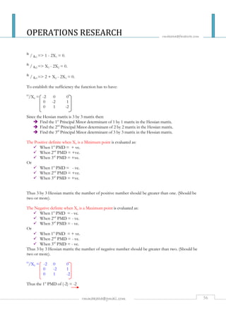
![OPERATIONS RESEARCH
rmakaha@facebook.com
Thus the 2nd PMD of –2 0
0 -2
rmmakaha@gmail.com 57
= (-2 * -2) – (0 * 0)
= 4
The 3rd PMD = -2 0 0
0 -2 1
0 1 -2
= -2 –2 1 - 0 0 1 + 0 0 -2
1 -2 0 -2 0 1
= -2 {(-2 * -2) – (1 * 1)} – 0 (0 – 0) + 0 (0 – 0)
= - 2 (3)
= - 6
Thus the PMD is equal to –2, 4 and –6 and H/X0 is negative definite and X0 = (½, 2/3, 4/3) represents a
Maximum point.
Question 2:
Given f(X1, X2, X3) =(-X1 + 2X3 - X2X3 + X2
1+ X2
2 - X2
3)
i. Find the gradient vector for X0 i.e. Ñf (X0) = 0.
ii. Determine the nature of the turning points using Hessian Matrix.
Solution:
The necessary condition (gradient vector) Ñf (X0) = 0 is given by:
df / dx1 = -1 + 2X1 = 0.
-1 + 2X1 = 0. [1]
df / dx2 = -X3 + 2X2 = 0.
-X3 + 2X2 = 0. [2]
df / dx3 = 2 - X2 - 2X3 = 0.
2 - X2 - 2X3 = 0. [3]
(b) Finding X1 is given by -1 = 2X1
X1 = ½
(b) Equation 2 is given by -X3 + 2X2 = 0.
X3 = 2X2.
(c) On equation 3 where therefore substitute X3 with 2X2.
Thus 2 - X2 - 2X3 = 0.](https://image.slidesharecdn.com/operationsresearch-141109234626-conversion-gate01/85/OPERATIONS-RESEARCH-57-320.jpg)


![OPERATIONS RESEARCH
rmakaha@facebook.com
PROBABILITY DISTRIBUTION (CONTINUOUS RANDOM VARIABLES):
A random variable X that can be equal to any number in an interval, which can be either finite
or infinite length, is called a Continuous Random Variable.
PROBABILITY DENSITY FUNCTIONS:
There are 2 essential properties of Pdf:
Because probabilities cannot be negative. The integral of a function must be non-negative
for all choices of interval [a, b] i.e. f(x) = 0 for all values in the sample space for the
random variable X.
Since the probability associated with the entire sample space is always 1. The integral of
f(x) of the entire sample space = 1.
Question 1:
A continuous random variable has Pdf f(x) where f(x) = kx, 0= x = 4.
i. Find the value of constant k.
ii. Sketch y = f(x).
iii. Find P(1 = X = 2½).
2½[⅛x]∂x.
rmmakaha@gmail.com 87
Solution:
i. ∫ f(x) ∂x = 1.
all x
∫4 kx ∂x = 1.
0
[kx2/]4 = 1.
20
8k = 1
k = ⅛
ii. Sketch of y = f(x).
½ y = ⅛x
0 4
P(1= x = 2½) = ∫1
= [x2/16]1
2½
= 0.328](https://image.slidesharecdn.com/operationsresearch-141109234626-conversion-gate01/85/OPERATIONS-RESEARCH-87-320.jpg)
![OPERATIONS RESEARCH
rmakaha@facebook.com
Question 2:
A continuous random variable has Pdf f(x) where
Kx 0= x = 4.
f(x)= k(4 – x) 2= x = 4
0 otherwise
a) Find the value of constant k.
b) Sketch y = f(x).
rmmakaha@gmail.com 88
Solution:
D =∫a
b P ∂x + ∫a
b Q ∂x = 1.
2 kx ∂x + ∫2
=∫0
4 k(4 – x) ∂x = 1.
= [kx2/2]0
2 + [4xk - kx2/2]2
4 = 1.
= [4k/2] – [0] + {[16k - 16k/2] – [8k - 4k/2]} = 1.
[2k] + {[8k] – [6k]} = 1.
4k = 1
k = ¼
c. Sketch y = f(x).
X 0 1 2 3 4
Y 0 ¼ ½ ¾ 1
F(x) = kx.
X 2 3 4
Y ½ ¼ 0
F(x) = k(4 – x)
1
¾
½
¼
0 1 2 3 4](https://image.slidesharecdn.com/operationsresearch-141109234626-conversion-gate01/85/OPERATIONS-RESEARCH-88-320.jpg)
![OPERATIONS RESEARCH
rmakaha@facebook.com
EXPECTED VALUE OR MEAN (CONTINUOUS RANDOM VARIABLE):
For a continuous random variable X defined within finite interval [a, b] with continuous Pdf f(x)
then the expected value or mean is given by:
1 6/7 x2 ∂x + ∫1
1 + 6/7[2/3x3 – x4/4]1
rmmakaha@gmail.com 89
E(x) = ∫a
b x. f(x) ∂x
Question 3:
A continuous random variable has Pdf f(x) where
6/7x 0= x = 1.
f(x)= 6/7x(2 – x) 1= x = 2
0 otherwise
i. Find E(x).
ii. Find E(x2).
Solution:
D =∫a
b P ∂x + ∫a
b Q ∂x = 1.
E(x) = ∫a
b x. f(x) ∂x
E(x) = ∫0
2 6/7 x2(2 – x)∂x
= 6/7[x3/3]0
2
= 6/7[⅓] + 6/7{16/3 – 4 – (⅔ - ¼)}
= 6/7[5/4]
= 15/14
E(x2) = ∫a
b x2. f(x) ∂x
E(x2) = ∫0
1 6/7 x3 ∂x + ∫1
2 6/7 x3(2 – x)∂x
= 6/7[x4/4]0
1 + 6/7[x4/2 – x5/5]1
2
= 6/7[¼] + 6/7{8 - 32/5 – (½ - 1/5)}
= 6/7[31/20]
= 93/70](https://image.slidesharecdn.com/operationsresearch-141109234626-conversion-gate01/85/OPERATIONS-RESEARCH-89-320.jpg)
![OPERATIONS RESEARCH
rmakaha@facebook.com
VARIANCE AND STANDARD DEVIATION:
The variance and Standard Deviation associated with a continuous random variable X on the
sample space [a, b] is given by:
4 ⅛x2 ∂x
= ⅛[x3/3]0
b x2. f(x) ∂x
=∫0
rmmakaha@gmail.com 90
Var (x) = ∫a
b [x - E(x)]2 . f(x) ∂x or Var(x) = E(x2) - μ2 ∂x
and Standard deviation = √Var (x).
E(x) = μ.
Question 4:
A continuous random variable has Pdf f(x) where f(x) = ⅛x, 0= x= 4.
Find:
a) E(x).
b) E(x2).
c) Var (x).
d) The standard deviation of x.
e) Var(3x +2).
Solution:
i. E(x) = ∫a
b x. f(x) ∂x
E(x) = ∫0
4
= 8/3
ii. E(x2) = ∫a
4 ⅛x3 ∂x
= ⅛[x4/4]0
4
= ⅛(64)
= 8
iii. Var(x) = E(x2) - μ2 ∂x
= E(x2) - E2(x) ∂x
= 8 – (8/3)2
= 8/9](https://image.slidesharecdn.com/operationsresearch-141109234626-conversion-gate01/85/OPERATIONS-RESEARCH-90-320.jpg)


![OPERATIONS RESEARCH
rmakaha@facebook.com
2 PROPERTIES OF CDF:
rmmakaha@gmail.com 93
F(b) = ∫a
b f(x) ∂x = 1.
If f(x) is valid for -¥ = x = ¥ then F(t) = ∫-¥
t f(x) ∂x where the interval is taken
over all values of x = t.
The Cumulative distribution function is sometimes known as just as the distribution
function.
Question 6:
A continuous random variable has Pdf f(x) where f(x) = ⅛x, 0= x= 4.
Find:
i. The Cumulative distribution function F(x).
ii. Sketch y = F(x).
iii. Find P(0.3 =x= 1.8).
Solution:
i. F(t) = ∫a
t f(x) ∂x
t ⅛x ∂x
= ⅛[x2/2]0
F(t) = ∫0
t
= t2/16
F (t) = t2/16 0=t=4
NB: (1) F(4) = 42/16 = 1
0 x = 0.
F(x) = x2/16 0= x = 4
1 x = 4
ii. Sketch y = F(x).
X 0 1 2 3 4
Y 0 1/16 1/2 9/16 1](https://image.slidesharecdn.com/operationsresearch-141109234626-conversion-gate01/85/OPERATIONS-RESEARCH-93-320.jpg)

![OPERATIONS RESEARCH
rmakaha@facebook.com
t x/3∂x
t
rmmakaha@gmail.com 95
Solution:
i. Sketch y = f(x).
X 0 1 2
Y 0
X 2 3
Y 0
y = x/3
y =-2x/3 +2
0 1 2 3
ii. CDF = F(t) = ∫0
= [x2/6]0
t
= t2/6
F (t) = x2/6 0=x=2
NB: F (2) = 22/6 =
F(t) = F(2) + (Area under the curve y = -2x/3 +2 between 2 and t)
So
F(t) = F(2) + ∫2
t (-2x/3 +2) ∂x
= F(2) + [-x2/3 + 2x]2
= + {-t2/3 +2t – ( -4/3 + 4)}
= -t2/3 +2t – 2 2= t = 3
NB: F(2) = -9/3 + 6 – 2 = 1](https://image.slidesharecdn.com/operationsresearch-141109234626-conversion-gate01/85/OPERATIONS-RESEARCH-95-320.jpg)


![OPERATIONS RESEARCH
rmakaha@facebook.com
Question 9:
A continuous random variable X takes values in the interval 0 to 3.
It is given that P(X x) = a + bx3, 0 = x = 3.
i. Find the values of the constants a and b.
ii. Find the Cumulative distribution function F(x).
iii. Find the Probability density function f(x).
iv. Show that E(x) = 2.25.
v. Find the Standard deviation.
rmmakaha@gmail.com 98
Solution:
a. P(X x) = a + bx3, 0 = x = 3.
So P(X 0) = 1 and P(X 3) = 0.
i.e. a + b(0) = 1 and a + b(27) = 0
Therefore a = 1 and 1 + 27b = 0.
B = -1/27.
So P(X x) = 1 - x3/27, 0 = x = 3.
b. Now P(X = x) = x3/27 (CDF)
X3/27 0=x=3
F(x) =
1 x 3.
c. f(x) = d/∂x * F(x).
= d/∂x(x3/27).
= 3x2/27
= x2/9
b x. f(x) ∂x
=∫0
d. E(x) = ∫a
3 x. x2/9∂x
3 x3/27∂x
=∫0
3
= [x4/36]0
= 2.25](https://image.slidesharecdn.com/operationsresearch-141109234626-conversion-gate01/85/OPERATIONS-RESEARCH-98-320.jpg)
![OPERATIONS RESEARCH
rmakaha@facebook.com
3 x4/9∂x – 2.252.
1∂X [(XY + Y2/2 - XY2)]0
½∂X[(XY + Y2/2 - XY2)]0
½∂X[(¼X + 1/32 - 1/16X)]
rmmakaha@gmail.com 99
e. Var(x) = ∫a
b [x - E(x)]2 . f(x) ∂x = ∫a
b x2.f(x)∂x - E2(X)
=∫0
=[x5/45]0
3 - 5.0625.
= 0.3375
f. δ = √ Var (x).
= √ 0.3375
= 0.581
RELATIONSHIPS AMONG PROBABILITY DISTRIBUTIONS:
JOINT PROBABILITY DISTRIBUTION:
Question 1:
2(X + Y - 2XY)0= X=1, 0= Y=1
Given f(X, Y) = 0 Otherwise
i. Show that this is a PDF.
ii. Find P(0 = X =½), (0 = Y =¼).
iii. Find CDF.
Solution:
a) =∫a
b∂X∫a
b∂Y
1∂X∫0
=∫0
1∂Y [2(X + Y - 2XY)]
= 2∫0
1
1∂X [(X + ½ - X)]
= 2∫0
= 2[(X2/2 + ½X - X2/2)]0
1
= 2[½ + ½ - ½]
= 2 * ½
= 1
b) =∫a
b∂X∫a
b∂Y
½∂X∫0
=∫0
¼∂Y [2(X + Y - 2XY)]
= 2∫0
¼
= 2∫0
½∂X[(3/16X + 1/32)]
= 2∫0
= 2[(3/32X2 + 1/32X)] 0
½](https://image.slidesharecdn.com/operationsresearch-141109234626-conversion-gate01/85/OPERATIONS-RESEARCH-99-320.jpg)
![OPERATIONS RESEARCH
rmakaha@facebook.com
x∂U[(UV + V2/2 - UV2)]0
x∂U[(UY + Y2/2 - UY2)]
rmmakaha@gmail.com 100
= 2[(3/128 + 1/64)]
= 2 * 5/128
= 5/64
c) F(u, v) =∫a
b∂u∫a
b∂v
x∂U∫0
=∫0
y∂V[2(U + V – 2UV)]
= 2∫0
y
= 2∫0
= 2[(YU2/2 + UY2/2 - U2X2/2)]0
X
= 2[(X2Y/2 + XY2/2 - X2X2/2)]
= X2Y + XY2 - X2X2
NB: Given CDF to get PDF we differentiate the function.
Given PDF to get CDF we integrate the function.
Given a PDF to prove that it is a PDF integrate until the answer is 1.
Given PDF the marginal distribution is found by integrating.
Given CDF the marginal distribution is found by differentiating.
Question 1:
Given the CDF = x2 + 3xyz + z.
Find the corresponding PDF.
Solution:
To get the corresponding PDF we differentiate with respect to x, y, z.
f(x, y, z) =x2 + 3xyz + z
= d/∂x(2x + 3yz).
= d/∂y(3z).
= d/∂z (3).
= 3](https://image.slidesharecdn.com/operationsresearch-141109234626-conversion-gate01/85/OPERATIONS-RESEARCH-100-320.jpg)


![OPERATIONS RESEARCH
rmakaha@facebook.com
Ok, the question on your mind is probably How the [expletive deleted] did you come up with those
numbers?. Let's take a look at a couple of examples.
rmmakaha@gmail.com 103
Demand is 50, buy 60:
They bought 60 at $65 each for $3900. That is -$3900 since that is money they spent. Now,
they sell 50 bicycles at $100 each for $5000. They had 10 bicycles left over at the end of the
season, and they sold those at $45 each of $450. That makes $5000 + 450 - 3900 = $1550.
Demand is 70, buy 40:
They bought 40 at $67 each for $2680. That is a negative $2680 since that is money they
spent. Now, they sell 40 bicycles (that's all they had) at $100 each for $4000. The other 30
customers that wanted a bicycle, but couldn't get one, left mad and Zed and Adrian lost $5
in goodwill for each of them. That's 30 customers at -$5 each or -$150. That makes $4000 -
2680 - 150 = $1170.
Opportunistic Loss Table
The opportunistic loss (regret) table is calculated from the payoff table. It is only needed for the
minimax criteria, but let's go ahead and calculate it now while we're thinking about it.
The maximum payoffs under each state of nature are shown in bold in the payoff table above. For
example, the best that Zed and Adrian could do if the demand was 30 bicycles is to make $770.
Each element in the opportunistic loss table is found taking each state of nature, one at a time, and
subtracting each payoff from the largest payoff for that state of nature. In the way we have the table
written above, we would subtract each number in the row from the largest number in the row.
Action
State of Nature Buy 20 Buy 40 Buy 60 Buy 80
Demand 10 0 380 700 1020
Demand 30 220 0 320 640
Demand 50 1100 280 0 320
Demand 70 1980 1160 280 0
Remember that the numbers in this table are losses and so the smaller the number, the better.
Expected Value Criterion
Compute the expected value for each action.
For each action, do the following: Multiply the payoff by the probability of that payoff occurring.
Then add those values together. Matrix multiplication works really well for this as it multiplied pairs
of numbers together and adds them. If you place the probabilities into a 1x4 matrix and use the 4x4
matrix shown above, then you can multiply the matrices to get a 1x4 matrix with the expected value
for each action.](https://image.slidesharecdn.com/operationsresearch-141109234626-conversion-gate01/85/OPERATIONS-RESEARCH-103-320.jpg)


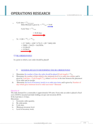


![OPERATIONS RESEARCH
rmakaha@facebook.com
Question 7:
The following is an illustration of a company with a simple manual reorder level system.
Normal Usage = 110 per day.
Minimum Usage = 50 per day.
Maximum Usage = 140 per day.
Lead time = 25 – 30 days.
EOQ = 5000
Using the above data calculate the various control levels i.e.
Reorder level.
Minimum Usage.
Maximum Usage. [20 marks].
rmmakaha@gmail.com 154
Solution:
a) Reorder Level = Maximum Usage * Maximum Lead time.
= 140 * 30
= 4200 units
b) Minimum Level = Reorder Level – (Average Lead time * Normal Usage)
= 4200 – (27.5 * 110)
= 4200 – 3025
= 1175 units
c) Maximum Level = Reorder Level + EOQ – (Min Lead time * Min Usage)
= 4200 + 5000 – (25 * 50)
= 7950
Question 8:
The following is an illustration of a company with a simple manual reorder level system.
Normal Usage = 560 per day.
Minimum Usage = 250 per day.
Maximum Usage = 750 per day.
Lead time = 15 – 20 days.
EOQ = 10000
Using the above data calculate the various control levels i.e.
Reorder level.
Minimum Usage.
Maximum Usage. [20 marks].
Solution:
a) Reorder Level = Maximum Usage * Maximum Lead time.
= 750 * 20
= 15000 units](https://image.slidesharecdn.com/operationsresearch-141109234626-conversion-gate01/85/OPERATIONS-RESEARCH-154-320.jpg)


![OPERATIONS RESEARCH
rmakaha@facebook.com
For the third correlation shows that there is no correlation existing between salary and age of an
employee. For non-linear correlation it suggests that quantity produced and efficiency are correlated but
not linearly.
Given two sets of data represented by the variables X and Y the Product Moment
Correlation Coefficient is given by:
r = Σ (X - r) (Y – Ý)
Ö Σ (X - r)2 * (Y – Ý)2
rmmakaha@gmail.com 157
OR
n ΣXY - ΣX * ΣY
r =
2 2 2 2
[n Σ X - (ΣX)] [n Σ Y - (ΣY)]
Question 1:
Calculate r for the data given below:
X 15 24 25 30 35 40 45 65 70 75
Y 60 45 50 35 42 46 28 20 22 15
Solution:
X Y XY X2 Y2
15 60 900 225 3600
24 45 1080 576 2025
25 50 1250 625 2500
30 35 1050 900 1225
35 42 1470 1225 1764
40 46 1840 1600 2116
45 28 1260 2025 784
65 20 1300 4225 400
70 22 1540 4900 484
75 15 1125 5625 225
424 363 12835 21926 15123](https://image.slidesharecdn.com/operationsresearch-141109234626-conversion-gate01/85/OPERATIONS-RESEARCH-157-320.jpg)
![OPERATIONS RESEARCH
rmakaha@facebook.com
n ΣXY - ΣX · ΣY
rmmakaha@gmail.com 158
r =
2 2 2 2
[n Σ X - (ΣX)] [n Σ Y - (ΣY)]
10 * 12835 - 424 * 363
r =
10* 21926 - 179776 * 10 * 15123 - 131769
128350 - 153912
r =
39484 * 19461
- 25562
r =
27719.9959
r = - 0.922150238 r = - 0.92
Question 2:
Calculate r for the data given below:
X 1 2 3 6 5 6
Y 5 10.5 15.5 25 16 22.5
Solution:
X Y XY X2 Y2
1 5 5 1 25
2 10.5 21 4 110.25
3 15.5 46.5 9 240.25
4 25 100 16 625
5 16 80 25 256
6 22.5 135 36 506.25
21 94.5 387.5 91 1762.75](https://image.slidesharecdn.com/operationsresearch-141109234626-conversion-gate01/85/OPERATIONS-RESEARCH-158-320.jpg)
![OPERATIONS RESEARCH
rmakaha@facebook.com
n ΣXY - ΣX * ΣY
rmmakaha@gmail.com 159
r =
2 2 2 2
[n Σ X - (ΣX)] [n Σ Y - (ΣY)]
6 * 387.5 - 21 * 94.5
r =
6* 91 - 441 * 6 * 1762.75 – 8930.25
2325 – 1984.5
r =
546 - 441 * 10576 – 8930.25
340.5
r =
415.7598467
r = 0.819
(B) THE SPEARMAN’S RANK CORRELATION COEFFICIENT:
When two sets of data are given positions or ranked, we use Spearman’s Rank Correlation Coefficient
represented by R. It is given by:
R = 1 - 6 Σd2
n(n2 -1)
Where d = difference between pairs of ranked values.
n = number of pairs of ranking.
1 = is an independent number.
Question 2:
A group of eight students were tested in Maths and English and the ranking in the two subjects are
given below:
Student A B C D E F G H
Maths 2 7 6 1 4 3 5 8
English 3 6 4 2 5 1 8 7](https://image.slidesharecdn.com/operationsresearch-141109234626-conversion-gate01/85/OPERATIONS-RESEARCH-159-320.jpg)


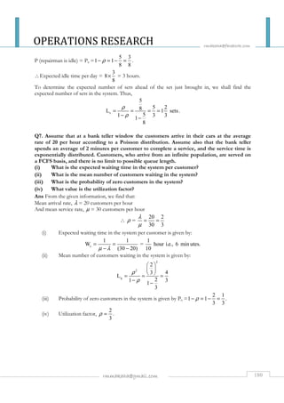
![OPERATIONS RESEARCH
rmakaha@facebook.com
(i) What is the probability that there is no customer in the counter (i.e. the system is
= =
1 P P P 1 1 1 1
-
rmmakaha@gmail.com 179
idle)?
(ii) What is the probability that there are more than 2 customers in the counter?
(iii) What is the probability that there is no customer waiting to be served?
(iv) What is the probability that a customer is being served and nobody is waiting?
Ans From the given information, we find that:
Mean arrival rate, l = 12 customers per hour
And mean service rate, m = 30 customers per hour
12
= 0.4
30
r l
m
(i) P (system is idle) = P0 = 1- r = 1- 0.4 = 0.6 .
(ii) P(n2) = 1–P(n£2)
[ ]
( ) ( )
( ) ( )
2
0 1 2
2
2
2
n 1
1 1 1
1 1 1
1 1 0.4 1 0.4 0.4
1 0.6 1.56
1 0.936
0.064
Also,P( n)
P( 2)
l l l l l
m m m m m
l l l
m m m
r r r
r +
= - + + = - - + - + -
= - - + +
= - - + +
= - - + +
= - ´
= -
=
=
= 0.42+1 = 0.43 = 0.064
(iii) P(no customer waiting to be served) = P0 + P1
= 0.6 + 0.24 = 0.84
(iv) P (a customer is being served and none is waiting) = P1 = 1 l l
m m
=r (1- r )= 0.4 x
0.6 = 0.24.
Q6. A TV repairman finds that the time spent on his job has an exponential distribution
with mean 30 minutes. If he repairs sets in the order in which they come and if the arrival of
sets is approximately Poisson with an average rate of 10 per 8-hour day, what is his expected
idle time each day? How many jobs are ahead of the set just brought in?
Ans From the given information, we find that:
Mean arrival rate, l = 10 sets per day.
And mean service rate, m = 16 sets per day.
10 5
=
= =
16 8
r l
m](https://image.slidesharecdn.com/operationsresearch-141109234626-conversion-gate01/85/OPERATIONS-RESEARCH-179-320.jpg)

The document covers various numerical methods in operations research, including the Newton-Raphson method for solving polynomial equations, the Trapezium rule and Simpson's rule for estimating integrals, and the Maclaurin series for function expansions. It also explains linear programming techniques for optimizing resource allocation in businesses and describes the simplex method for solving linear programming problems. Real-world examples are provided to illustrate the application of these methods in maximizing profits or minimizing costs.