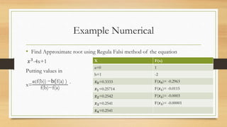
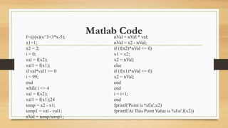
This document describes the False Position Method for finding the roots of equations. The method uses linear interpolation to estimate the root between two initial guesses that bracket it. It improves on the bisection method by choosing a "false position" where the line between the guesses crosses the x-axis, rather than the midpoint. The false position formula is derived using similar triangles. An example applying the method to find a root of x^3 - 2x - 3 = 0 is shown. The merits of the false position method are faster convergence compared to bisection, while the demirits are possible non-monotonic convergence and lack of precision guarantee.
Regula Falsi or False Position Method is one of the iterative (bracketing) Method for solving root(s) of nonlinear equation under Numerical Methods or Analysis.
The document describes the Regula Falsi method, a numerical method for estimating the roots of a polynomial function. The Regula Falsi method improves on the bisection method by using a value x that replaces the midpoint, serving as a new approximation of a root. An example problem demonstrates applying the Regula Falsi method to find the root of a function between 1 and 2 to within 3 decimal places. Limitations of the method include potential slow convergence, reliance on sign changes to find guesses, and inability to detect multiple roots.
This document discusses several numerical analysis methods for finding roots of equations or solving systems of equations. It describes the bisection method for finding roots of continuous functions, the method of false positions for approximating roots between two values with opposite signs of a function, Gauss elimination for transforming a system of equations into triangular form, Gauss-Jordan method which further eliminates variables in equations below, and iterative methods which find solutions through successive approximations rather than direct computation.
This document discusses Joseph-Louis Lagrange and interpolation. It provides:
1) A brief biography of Joseph-Louis Lagrange, an Italian mathematician who made significant contributions to calculus and probability.
2) A definition of interpolation as producing a function that matches given data points exactly and can be used to approximate values between points.
3) An explanation of Lagrange's interpolation formula for finding a polynomial that fits a set of data points, including an example of applying the formula.
Integration is used in physics to determine rates of change and distances given velocities. Numerical integration is required when the antiderivative is unknown. It involves approximating the definite integral of a function as the area under its curve between bounds. The Trapezoidal Rule approximates this area using straight lines between points, while Simpson's Rule uses quadratic or cubic functions, achieving greater accuracy with fewer points. Both methods involve dividing the area into strips and summing their widths multiplied by the function values at strip points.
The false position method is a root-finding algorithm that uses linear interpolation to estimate the root of a function. It improves upon the bisection method by using the function values at the endpoints of the interval rather than just their signs. The method chooses the intercept of the secant line through the two endpoints as the next approximation of the root, and continues iteratively narrowing the interval until the root is found.
The False-Position Method is an iterative root-finding algorithm that improves upon the bisection method. It uses the slope of a line between two points to estimate a new root, rather than always bisecting the interval. Given an initial interval where the function changes sign, it calculates a new x-value at the intersection of the x-axis and a line through two existing points. It then chooses a new interval based on where the function changes sign again. The method is similar to bisection but uses a different formula to calculate the new estimate. An example finds a root of 3x + sin(x) - exp(x) = 0 between 0 and 0.5, converging to a solution of approximately 0.
The bisection method is an iterative method for finding the root of a non-linear equation. It works by repeatedly bisecting an interval and narrowing in on the root. The method takes an initial interval [a,b] where the function values at the endpoints have opposite signs, indicating a root exists in the interval. It then computes the midpoint m of the interval. If the function values at m and a have the same sign, the root must lie in [m,b], otherwise it is in [a,m]. This process of bisecting the interval continues until the interval size is sufficiently small. The method is simple to implement and requires only one function evaluation per iteration but converges slowly.
The document discusses the Mean Value Theorem, which states that if a function f(x) is continuous on the closed interval [a,b] and differentiable on the open interval (a,b), then there exists some value c in (a,b) such that:
f(b) - f(a) = f'(c)(b - a)
In other words, there is at least one point where the slope of the tangent line equals the slope of the secant line between points a and b. The document provides examples and illustrations to demonstrate how to apply the Mean Value Theorem.
This lecture contains Newton Raphson Method working rule, Graphical representation, Example, Pros and cons of this method and a Matlab Code.
Explanation is available here: https://www.youtube.com/watch?v=NmwwcfyvHVg&lc=UgwqFcZZrXScgYBZPcV4AaABAg
The document describes the bisection method, also known as interval halving, for finding roots of nonlinear equations. It discusses Bolzano's theorem which guarantees a root between intervals where the function changes sign. The bisection algorithm iteratively halves intervals and chooses the sub-interval based on the function value. The number of iterations needed for a given tolerance can be determined from the log formula provided. An example finds the root of an exponential equation in 10 iterations to within tolerance 10^-3.
The secant method is a root-finding algorithm that uses successive secants of a function to linearly approximate the root. It requires two initial guesses, x0 and x1, to construct a secant line through the points (x0, f(x0)) and (x1, f(x1)). The x-intercept of this line provides the next approximation x2. Repeating this process iteratively refines the approximation until the root is found to within a desired precision. The secant method converges faster than bisection near roots and does not require evaluating derivatives, but it may fail to converge for some functions.
The document discusses the bisection method for finding roots of equations. It begins by defining the bisection method as a root finding technique that repeatedly bisects an interval and selects a subinterval containing the root. It notes that while simple and robust, the bisection method converges slowly. The document then provides the step-by-step algorithm for implementing the bisection method and works through an example of finding the root of f(x) = x^2 - 2 between 1 and 2. It concludes by presenting the bisection method code in C++.
The document describes the bisection method for finding roots of equations. It provides an introduction to the bisection method and its graphical representation. It also presents the algorithm, a C program implementing the method, and examples finding roots of polynomial and trigonometric equations using bisection.
- Rolle's theorem states that if a function f(x) is continuous on a closed interval [a,b] and differentiable on the open interval (a,b), with f(a) = f(b), then there exists at least one value c in (a,b) where the derivative f'(c) = 0.
- The mean value theorem states that if a function f(x) is continuous on a closed interval [a,b] and differentiable on the open interval (a,b), then there exists a value c in (a,b) such that the average rate of change of f over the interval [a,b] equals the instantaneous rate of change
The secant method is a root-finding algorithm that uses successive secant lines to approximate the root of a function. It can be considered a finite difference approximation of Newton's method. The secant method converges faster than linear but not quite quadratically, and only requires evaluating the function at each iteration rather than both the function and its derivative like Newton's method. Therefore, the secant method may be more efficient in some cases, though it does not always guarantee convergence like Newton's method.
The document provides information about the bisection method for finding roots of non-linear equations. It defines the bisection method, outlines its basis and key steps, and provides an example of using the method to find the depth at which a floating ball is submerged in water. Over 10 iterations, the bisection method converges on an estimated root of 0.06241 for the example equation, with 2 significant digits found to be correct after the final iteration. The document also discusses an application of using the bisection method to find resistance of a thermistor at a given temperature.
This presentation is a part of Computer Oriented Numerical Method . Newton-Cotes formulas are an extremely useful and straightforward family of numerical integration techniques.
This document discusses approximation and round-off error in engineering. It defines approximation as using an inexact value when the exact value is unknown or difficult to obtain. Approximations introduce errors from measurements in the real world. There are two main types of errors - truncation error from dropping digits during approximations, and rounding error from representing numbers with a fixed number of significant figures. The absolute error is the difference between the true and approximate values, while relative error is the percentage difference between the absolute error and true value.
The document discusses the bisection method for finding real roots of equations. It provides the step-by-step algorithm for applying the bisection method. The key steps are: (1) find two values a and b where the function has opposite signs, (2) compute the midpoint x0 between a and b and evaluate the function there, (3) replace either a or b with x0 depending on whether f(x0) is positive or negative, and (4) repeat until the desired accuracy is reached. The document includes an example of applying the bisection method to find the root of the equation f(x) = x^3 - 2x - 5 between 2 and 3.
The document discusses numerical methods for solving algebraic and transcendental equations. It describes direct and iterative methods. Bisection, regula falsi, and Newton Raphson are iterative root-finding algorithms explained in detail with examples. The order of convergence of iterative methods is defined as the rate at which error decreases between successive approximations. The document serves as seminar material on engineering mathematics covering numerical solutions of equations.
This document discusses Newton's forward and backward difference interpolation formulas for equally spaced data points. It provides the formulations for calculating the forward and backward differences up to the kth order. For equally spaced points, the forward difference formula approximates a function f(x) using its kth forward difference at the initial point x0. Similarly, the backward difference formula approximates f(x) using its kth backward difference at x0. The document includes an example problem of using these formulas to estimate the Bessel function and exercises involving interpolation of the gamma function and exponential function.
Computer Oriented Numerical Analysis
What is interpolation?
Many times, data is given only at discrete points such as .
So, how then does one find the value of y at any other value of x ?
Well, a continuous function f(x) may be used to represent the data values with f(x) passing through the points (Figure 1). Then one can find the value of y at any other value of x .
This is called interpolation
Newton’s Divided Difference Formula:
To illustrate this method, linear and quadratic interpolation is presented first.
Then, the general form of Newton’s divided difference polynomial method is presented.
This presentation gives a brief idea about Interpolation. Methods of interpolating with equally/unequally spaced intervals. Please note that not all the methods are being covered in this presentation. Topics like extrapolation and inverse interpolation have also been kept aside for another ppt.
Fortran is a general-purpose programming language, mainly intended for mathematical computations in
science applications
this chapter is the third chapter
The document summarizes numerical methods for finding the roots of equations, including the Newton-Raphson method, secant method, false position method, and methods for handling repeated roots.
The Newton-Raphson method uses the tangent line to iteratively find better approximations to the root. It has quadratic convergence but may diverge for repeated roots. The secant method approximates the derivative using two points to overcome issues with the Newton-Raphson method. The false position method uses linear interpolation in each interval to home in on the root. For repeated roots, the modified Newton-Raphson method solves for the roots of a related function to ensure convergence.
Analysis for engineers _roots_ overeruptionuttamna97
This document discusses numerical methods for finding roots of equations. It introduces graphical methods for simple functions, as well as bracketing methods that use two initial guesses to bracket the root. The bisection method and false position (regula falsi) method are explained in detail. Bisection takes the average of the bracketing guesses at each iteration, while false position uses linear interpolation. Examples are provided to illustrate applying both methods to example functions and comparing their rates of convergence.
The document provides the steps to solve a multi-part calculus problem involving derivatives, tangent lines, and circles. It determines the derivative of two functions f(x) and g(x), finds the equations of the tangent lines at specific x-values, identifies the intersection points of the tangent lines, and uses those intersection points as the centers of three circles with a radius of 5 to write the equations of the circles.
The document provides the steps to solve a multi-part calculus problem. It involves finding the derivative of two functions, determining the equations of tangent lines to those functions at given points, finding the intersection points of those tangent lines, and using those intersection points to write the equations of three circles with a radius of 5.
The document defines and explains key concepts regarding quadratic functions including:
- The three common forms of quadratic functions: general, vertex, and factored form
- How to find the x-intercepts, y-intercept, and vertex of a quadratic function
- Methods for solving quadratic equations including factoring, completing the square, and the quadratic formula
- How to graph quadratic functions by identifying intercepts and the vertex
The document introduces numerical methods for finding the roots or zeros of equations of the form f(x) = 0, where f(x) is an algebraic or transcendental function. It focuses on the bisection method, also called the Bolzano method, which uses interval bisection to bracket the root between two values where f(x) has opposite signs. The method iteratively narrows down the interval to find the root to within a specified tolerance. Several examples demonstrate applying the bisection method to find roots of polynomial, logarithmic, and trigonometric equations.
1. The document discusses function notation and evaluating functions algebraically. It provides examples of defining functions using f(x) = expression notation and evaluating functions at given values of x by substituting those values into the function expression.
2. Key steps shown include defining functions using symbols like f, g, and h; substituting values for x in functions defined as f(x) = expression; and evaluating functions at values, expressions, or functions of x following algebraic rules like distributing operations.
3. Examples evaluate functions at values like f(6), expressions like f(x+1), and functions of x like f(-x) to demonstrate the process of substituting the appropriate value for x and simplifying
This document discusses the continuity of functions. It defines a continuous function as one where the limit of the function as x approaches c exists and is equal to the value of the function at c. It also describes three types of discontinuity: removable, essential, and infinite. Examples are provided to demonstrate determining if a function is continuous at a given point by checking if the three conditions for continuity are met.
PRESENT.pptx this paper will help the nextseidnegash1
This document discusses the fixed point iteration method for finding approximate solutions to nonlinear equations. It begins with an introduction to roots of nonlinear equations and converting them to a fixed point problem. It then presents the fixed point iteration method theorem and algorithm. Examples are provided to demonstrate applying the method to find the roots of equations up to four decimal places. The document concludes by noting the method can be implemented using loops in code and is useful for finding real roots expressed as infinite series.
This document discusses evaluating functions and operations on functions. It provides examples of evaluating functions at given points by substituting the point value for the variable in the function definition and simplifying. Some key points made include:
- Function notation like f(x) identifies the function and indicates the variable it is in terms of
- To evaluate a function at a point, substitute the point value for the variable and simplify
- Functions can be evaluated using algebraic expressions by substituting the expression for the variable
- Examples are provided of evaluating various functions at given points or expressions
ppt.pptx fixed point iteration method noseidnegash1
The document discusses the fixed point iteration method, which is a numerical method used to find approximate solutions to algebraic and transcendental equations. It presents the theorems and algorithm of the fixed point iteration method, and provides examples of its applications. Some key points covered include expressing equations in the form x=g(x) such that the derivative is less than 1, using successive approximations xn=g(xn-1) to generate a converging sequence, and illustrating the geometric interpretation of the method graphically. The document concludes that fixed point theory has many applications in mathematics.
The document discusses quadratic functions and their zeros. It provides examples of finding the zeros of quadratic functions by factoring, completing the square, and using the quadratic formula. It also gives examples of writing the equation of a quadratic function given its zeros or given properties like the vertex and y-intercept. Methods discussed include using the fact that the zeros are the roots of the corresponding equation, and substituting known point values into the quadratic formula.
Linear approximations and_differentialsTarun Gehlot
The document discusses linear approximations and differentials. It explains that a linear approximation uses the tangent line at a point to approximate nearby values of a function. The linearization of a function f at a point a is the linear function L(x) = f(a) + f'(a)(x - a). Several examples are provided of finding the linearization of functions and using it to approximate values. Differentials are also introduced, where dy represents the change along the tangent line and ∆y represents the actual change in the function.
This document describes three approximation methods for integrals - the Midpoint Rule, Trapezoidal Rule, and Simpson's Rule. It provides the formulas for computing each approximation using n subintervals and estimates the error bounds. It then works through an example problem in detail, applying each method to compute the integral from 1 to 5 of 1/x dx and determining the necessary number of subintervals to achieve an accuracy of 0.01. Simpson's Rule is identified as the most efficient method.
This document discusses different numerical methods for finding the roots of equations, including the bisection method, false position method, and Newton-Raphson method. It provides details on how the bisection method works, including defining an interval where the solution lies and bisecting that interval recursively until the approximate root is found. An example of using the bisection method to find the root of an equation is shown. The false position method is described as similar but using the slope of a line between two points to get a better first approximation than bisection. Newton-Raphson is also introduced but not explained in detail.
The document defines quadratic functions and discusses their various forms, including general, vertex, and factored forms. It also covers solving quadratic equations using methods like the quadratic formula, factoring, and completing the square. Additionally, it discusses key features of quadratic graphs like x-intercepts, y-intercepts, the vertex, and concavity. Examples are provided to illustrate finding these features and graphing parabolas.
The secant method is a root-finding algorithm that uses successive secant lines to converge on a root of an equation. It begins with two initial points and finds where the secant line between those points intersects the x-axis. It then uses the intersection point as the next estimate and draws a new secant line. This process repeats until the estimate converges within a specified tolerance of the root. The secant method requires only function evaluations, unlike other methods that also require derivative evaluations. However, it may not always converge and provides no error bounds for the estimates.
The document discusses numerical methods for approximating integrals and solving non-linear equations. It introduces the trapezium rule for approximating integrals and provides examples of using the rule. It then discusses iterative methods like the iteration method and Newton-Raphson method for finding approximate roots of non-linear equations, providing examples of applying each method. The objectives are to enable students to use the trapezium rule and understand solving non-linear equations using iterative methods.
Similar to False Point Method / Regula falsi method (20)
Advanced control scheme of doubly fed induction generator for wind turbine us...IJECEIAES
This paper describes a speed control device for generating electrical energy on an electricity network based on the doubly fed induction generator (DFIG) used for wind power conversion systems. At first, a double-fed induction generator model was constructed. A control law is formulated to govern the flow of energy between the stator of a DFIG and the energy network using three types of controllers: proportional integral (PI), sliding mode controller (SMC) and second order sliding mode controller (SOSMC). Their different results in terms of power reference tracking, reaction to unexpected speed fluctuations, sensitivity to perturbations, and resilience against machine parameter alterations are compared. MATLAB/Simulink was used to conduct the simulations for the preceding study. Multiple simulations have shown very satisfying results, and the investigations demonstrate the efficacy and power-enhancing capabilities of the suggested control system.
Literature Review Basics and Understanding Reference Management.pptxDr Ramhari Poudyal
Three-day training on academic research focuses on analytical tools at United Technical College, supported by the University Grant Commission, Nepal. 24-26 May 2024
Embedded machine learning-based road conditions and driving behavior monitoringIJECEIAES
Car accident rates have increased in recent years, resulting in losses in human lives, properties, and other financial costs. An embedded machine learning-based system is developed to address this critical issue. The system can monitor road conditions, detect driving patterns, and identify aggressive driving behaviors. The system is based on neural networks trained on a comprehensive dataset of driving events, driving styles, and road conditions. The system effectively detects potential risks and helps mitigate the frequency and impact of accidents. The primary goal is to ensure the safety of drivers and vehicles. Collecting data involved gathering information on three key road events: normal street and normal drive, speed bumps, circular yellow speed bumps, and three aggressive driving actions: sudden start, sudden stop, and sudden entry. The gathered data is processed and analyzed using a machine learning system designed for limited power and memory devices. The developed system resulted in 91.9% accuracy, 93.6% precision, and 92% recall. The achieved inference time on an Arduino Nano 33 BLE Sense with a 32-bit CPU running at 64 MHz is 34 ms and requires 2.6 kB peak RAM and 139.9 kB program flash memory, making it suitable for resource-constrained embedded systems.
International Conference on NLP, Artificial Intelligence, Machine Learning an...gerogepatton
International Conference on NLP, Artificial Intelligence, Machine Learning and Applications (NLAIM 2024) offers a premier global platform for exchanging insights and findings in the theory, methodology, and applications of NLP, Artificial Intelligence, Machine Learning, and their applications. The conference seeks substantial contributions across all key domains of NLP, Artificial Intelligence, Machine Learning, and their practical applications, aiming to foster both theoretical advancements and real-world implementations. With a focus on facilitating collaboration between researchers and practitioners from academia and industry, the conference serves as a nexus for sharing the latest developments in the field.
Low power architecture of logic gates using adiabatic techniquesnooriasukmaningtyas
The growing significance of portable systems to limit power consumption in ultra-large-scale-integration chips of very high density, has recently led to rapid and inventive progresses in low-power design. The most effective technique is adiabatic logic circuit design in energy-efficient hardware. This paper presents two adiabatic approaches for the design of low power circuits, modified positive feedback adiabatic logic (modified PFAL) and the other is direct current diode based positive feedback adiabatic logic (DC-DB PFAL). Logic gates are the preliminary components in any digital circuit design. By improving the performance of basic gates, one can improvise the whole system performance. In this paper proposed circuit design of the low power architecture of OR/NOR, AND/NAND, and XOR/XNOR gates are presented using the said approaches and their results are analyzed for powerdissipation, delay, power-delay-product and rise time and compared with the other adiabatic techniques along with the conventional complementary metal oxide semiconductor (CMOS) designs reported in the literature. It has been found that the designs with DC-DB PFAL technique outperform with the percentage improvement of 65% for NOR gate and 7% for NAND gate and 34% for XNOR gate over the modified PFAL techniques at 10 MHz respectively.
2. Working Rule
• The Regula–Falsi Method is a numerical method for estimating the roots of a
polynomial f(x). A value x replaces the midpoint in the Bisection Method and serves as
the new approximation of a root of f(x). The objective is to make convergence
faster. Assume that f(x) is continuous.
• This method also known as CHORD METHOD ,, LINEAR INTERPOLATION and
method is one of the bracketing methods and based on intermediate value theorem
5. Algorithm
1.Find points a and b such that a < b and f(a) * f(b) < 0.
2.Take the interval [a, b] and determine the next value of x1.
3.If f(x1) = 0 then x1 is an exact root, else if f(x1) * f(b) < 0 then let a = x1,
else if f(a) * f(x1) < 0 then let b = x1.
4.Repeat steps 2 & 3 until f(xi) = 0 or |f(xi)| tolerance
6. Example Numerical
• Find Approximate root using Regula Falsi method of the equation
𝑥3-4x+1
Putting values in
x=
𝑎(f(b)) −b(f(a) )
f(b)−f(a)
`
X F(x)
a=0 1
b=1 -2
𝑥0=0.3333 F(𝑥0)= -0.2963
𝑥1=0.25714 F(𝑥1)= -0.0115
𝑥2=0.2542 F(𝑥2)= -0.0003
𝑥3=0.2541 F(𝑥3)= -0.00001
𝑥4=0.2541
7. Pros and Cons
Advantages
• 1. It always converges.
• 2. It does not require the derivative.
• 3. It is a quick method.
Disadvantages
• 1. One of the interval definitions can get stuck.
• 2. It may slowdown in unfavourable situations.
8. Matlab Code
f=@(x)(x^3+3*x-5);
x1=1;
x2 = 2;
i = 0;
val = f(x2);
val1 = f(x1);
if val*val1 >= 0
i = 99;
end
while i <= 4
val = f(x2);
val1 = f(x1);24
temp = x2 - x1;
temp1 = val - val1;
nVal = temp/temp1;
nVal = nVal * val;
nVal = x2 - nVal;
if (f(x2)*nVal <= 0)
x1 = x2;
x2 = nVal;
else
if (f(x1)*nVal <= 0)
x2 = nVal;
end
end
i = i+1;
end
fprintf('Point is %fn',x2)
fprintf('At This Point Value is %fn',f(x2))