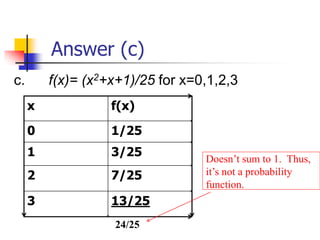
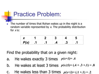
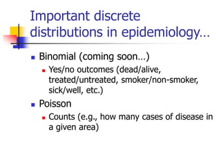
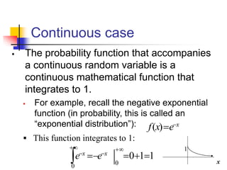
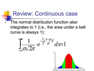
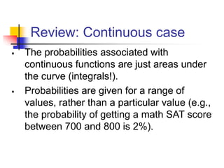
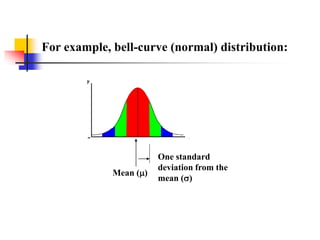
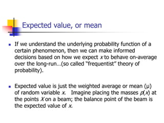
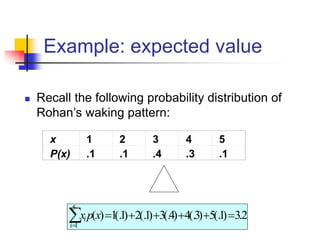
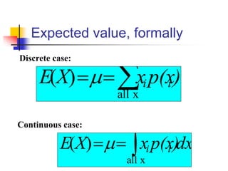
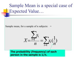
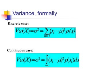
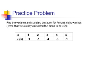
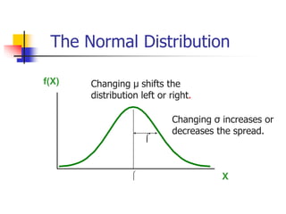
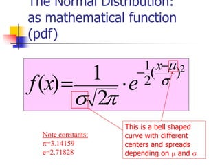
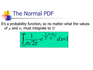
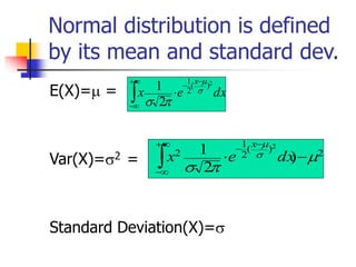
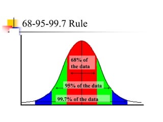
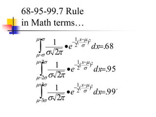
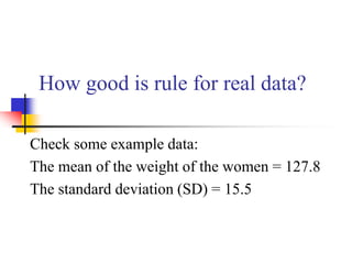
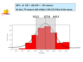
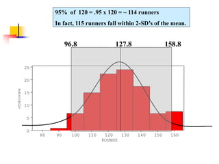
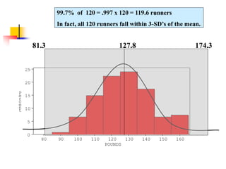
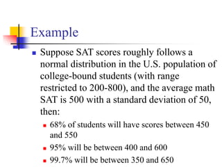
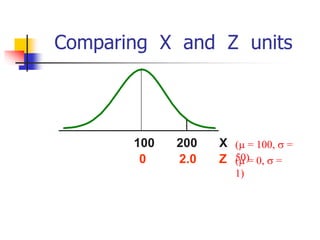
The document discusses probability distributions, defining random variables and their respective probability functions, including discrete and continuous types. It explains concepts like expected value and variance, using examples such as dice rolls and Rohan's night wakings to illustrate calculations related to probability. Additionally, it covers the normal distribution and the significance of its mean and standard deviation, presenting the 68-95-99.7 rule for understanding data spread.

1. Probability Distributions

2. Random Variable
• A random variable X takes on a defined set of
values with different probabilities.
• For example, if you roll a die, the outcome is random
(not fixed) and there are 6 possible outcomes, each of
which occur with probability one-sixth.
• For example, if you poll people about their voting
preferences, the percentage of the sample that responds
“Yes on Proposition 100” is a also a random variable (the
percentage will be slightly different every time you poll).
• Roughly, probability is how frequently we
expect different outcomes to occur if we
repeat the experiment over and over
(“frequentist” view)

3. Random variables can be
discrete or continuous
◼ Discrete random variables have a
countable number of outcomes
◼ Examples: Dead/alive, treatment/placebo,
dice, counts, etc.
◼ Continuous random variables have an
infinite continuum of possible values.
◼ Examples: blood pressure, weight, the
speed of a car, the real numbers from 1 to
6.

4. Probability functions
◼ A probability function maps the possible
values of x against their respective
probabilities of occurrence, p(x)
◼ p(x) is a number from 0 to 1.0.
◼ The area under a probability function is
always 1.

5. Discrete example: roll of a die
x
p(x)
1/6
1 4 5 6
2 3
 =
x
all
1
P(x)

6. Probability mass function (pmf)
x p(x)
1 p(x=1)=1/6
2 p(x=2)=1/6
3 p(x=3)=1/6
4 p(x=4)=1/6
5 p(x=5)=1/6
6 p(x=6)=1/6
1.0

7. Cumulative distribution function
(CDF)
x
P(x)
1/6
1 4 5 6
2 3
1/3
1/2
2/3
5/6
1.0

8. Cumulative distribution
function
x P(x≤A)
1 P(x≤1)=1/6
2 P(x≤2)=2/6
3 P(x≤3)=3/6
4 P(x≤4)=4/6
5 P(x≤5)=5/6
6 P(x≤6)=6/6

9. Examples
1. What’s the probability that you roll a 3 or less?
P(x≤3)=1/2
2. What’s the probability that you roll a 5 or higher?
P(x≥5) = 1 – P(x≤4) = 1-2/3 = 1/3

10. Practice Problem
Which of the following are probability functions?
a. f(x)=.25 for x=9,10,11,12
b. f(x)= (3-x)/2 for x=1,2,3,4
c. f(x)= (x2+x+1)/25 for x=0,1,2,3

11. Answer (a)
a. f(x)=.25 for x=9,10,11,12
Yes, probability
function!
x f(x)
9 .25
10 .25
11 .25
12 .25
1.0

12. Answer (b)
b. f(x)= (3-x)/2 for x=1,2,3,4
x f(x)
1 (3-1)/2=1.0
2 (3-2)/2=.5
3 (3-3)/2=0
4 (3-4)/2=-.5
Though this sums to 1,
you can’t have a negative
probability; therefore, it’s
not a probability
function.

13. Answer (c)
c. f(x)= (x2+x+1)/25 for x=0,1,2,3
x f(x)
0 1/25
1 3/25
2 7/25
3 13/25
Doesn’t sum to 1. Thus,
it’s not a probability
function.
24/25

14. Practice Problem:
◼ The number of times that Rohan wakes up in the night is a
random variable represented by x. The probability distribution
for x is:
x 1 2 3 4 5
P(x) .1 .1 .4 .3 .1
Find the probability that on a given night:
a. He wakes exactly 3 times
b. He wakes at least 3 times
c. He wakes less than 3 times
p(x=3)= .4
p(x3)= (.4 + .3 +.1) = .8
p(x<3)= (.1 +.1) = .2

15. Important discrete
distributions in epidemiology…
◼ Binomial (coming soon…)
◼ Yes/no outcomes (dead/alive,
treated/untreated, smoker/non-smoker,
sick/well, etc.)
◼ Poisson
◼ Counts (e.g., how many cases of disease in
a given area)

16. Continuous case
▪ The probability function that accompanies
a continuous random variable is a
continuous mathematical function that
integrates to 1.
▪ For example, recall the negative exponential
function (in probability, this is called an
“exponential distribution”): x
e
x
f −
=
)
(
1
1
0
0
0
=
+
=
−
=
+
−
+
−
 x
x
e
e
▪ This function integrates to 1:
x
1

17. Review: Continuous case
▪ The normal distribution function also
integrates to 1 (i.e., the area under a bell
curve is always 1):
1
2
1 2
)
(
2
1
=


+

−
−
−
dx
e
x





18. Review: Continuous case
▪ The probabilities associated with
continuous functions are just areas under
the curve (integrals!).
▪ Probabilities are given for a range of
values, rather than a particular value (e.g.,
the probability of getting a math SAT score
between 700 and 800 is 2%).

19. Expected Value and Variance
◼ All probability distributions are
characterized by an expected value
(=mean!) and a variance (standard
deviation squared).

20. For example, bell-curve (normal) distribution:
One standard
deviation from the
mean ()
Mean ()

21. Expected value, or mean
◼ If we understand the underlying probability function of a
certain phenomenon, then we can make informed
decisions based on how we expect x to behave on-average
over the long-run…(so called “frequentist” theory of
probability).
◼ Expected value is just the weighted average or mean (µ)
of random variable x. Imagine placing the masses p(x) at
the points X on a beam; the balance point of the beam is
the expected value of x.

22. Example: expected value
◼ Recall the following probability distribution of
Rohan’s waking pattern:

=
=
+
+
+
+
=
5
1
2
.
3
)
1
(.
5
)
3
(.
4
)
4
(.
3
)
1
(.
2
)
1
(.
1
)
(
i
i x
p
x
x 1 2 3 4 5
P(x) .1 .1 .4 .3 .1

23. Expected value, formally

=
=
x
all
)
( )
p(x
x
X
E i
i

Discrete case:
Continuous case:
dx
)
p(x
x
X
E i
i

=
=
x
all
)
( 

24. Sample Mean is a special case of
Expected Value…
Sample mean, for a sample of n subjects: =
)
1
(
1
1
n
x
n
x
X
n
i
i
n
i
i


=
=
=
=
The probability (frequency) of each
person in the sample is 1/n.

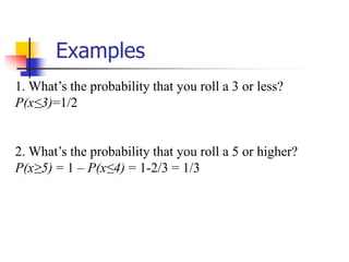
25. Variance/standard deviation
“The average (expected) squared
distance (or deviation) from the mean”
 −
=
−
=
=
x
all
2
2
2
)
(
]
)
[(
)
( )
p(x
x
x
E
x
Var i
i 


**We square because squaring has better properties than
absolute value. Take square root to get back linear average
distance from the mean (=”standard deviation”).

26. Variance, formally
 −
=
=
x
all
2
2
)
(
)
( )
p(x
x
X
Var i
i 

Discrete case:
Continuous case:



−
−
=
= dx
x
p
x
X
Var i
i )
(
)
(
)
( 2
2



27. Sample variance is a special
case…
The variance of a sample: s2 =
)
1
1
(
)
(
1
)
(
2
1
2
1
−
−
=
−
−


=
=
n
x
x
n
x
x N
i
i
N
i
i
Division by n-1 reflects the fact that we have lost a
“degree of freedom” (piece of information) because
we had to estimate the sample mean before we could
estimate the sample variance.

28. Practice Problem
A roulette wheel has the numbers 1 through
36, as well as 0 and 00. If you bet $1.00 that
an odd number comes up, you win or lose
$1.00 according to whether or not that event
occurs. If X denotes your net gain, X=1 with
probability 18/38 and X= -1 with probability
20/38.
◼ We already calculated the mean to be = -$.053.
What’s the variance of X?

29. Answer
Standard deviation is $.99. Interpretation: On average, you’re
either 1 dollar above or 1 dollar below the mean, which is just
under zero. Makes sense!
 −
=
x
all
2
2
)
( )
p(x
x i
i 

997
.
)
38
/
20
(
)
947
.
(
)
38
/
18
(
)
053
.
1
(
)
38
/
20
(
)
053
.
1
(
)
38
/
18
(
)
053
.
1
(
)
38
/
20
(
)
053
.
1
(
)
38
/
18
(
)
053
.
1
(
2
2
2
2
2
2
=
−
+
=
+
−
+
=
−
−
−
+
−
−
+
=
99
.
997
. =
=


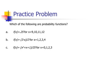
30. calculation formula!
2
x
all
2
x
all
2
)
(
)
(
)
( 
 −
=
−
= 
 )
p(x
x
)
p(x
x
X
Var i
i
i
i
Intervening algebra!
2
2
)]
(
[
)
( x
E
x
E −
=

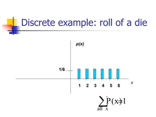
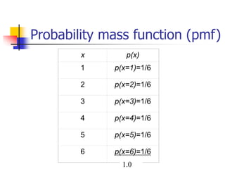
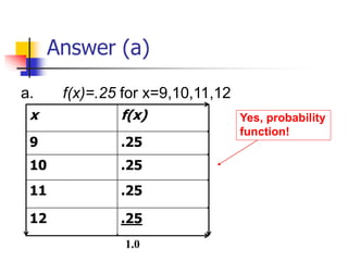
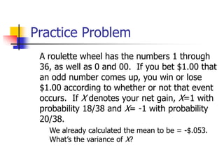
31. For example, what are the mean and
standard deviation of the roll of a die?
x p(x)
1 p(x=1)=1/6
2 p(x=2)=1/6
3 p(x=3)=1/6
4 p(x=4)=1/6
5 p(x=5)=1/6
6 p(x=6)=1/6
1.0
17
.
15
)
6
1
(
36
)
6
1
(
25
)
6
1
(
16
)
6
1
(
9
)
6
1
(
4
)
6
1
)(
1
(
)
(
x
all
2
2
=
+
+
+
+
+
=
= )
p(x
x
x
E i
i
5
.
3
6
21
)
6
1
(
6
)
6
1
(
5
)
6
1
(
4
)
6
1
(
3
)
6
1
(
2
)
6
1
)(
1
(
)
(
x
all
=
=
+
+
+
+
+
=
= )
p(x
x
x
E i
i
71
.
1
92
.
2
92
.
2
5
.
3
17
.
15
)]
(
[
)
(
)
( 2
2
2
2
=
=
=
−
=
−
=
=
x
x x
E
x
E
x
Var


x
p(x)
1/6
1 4 5 6
2 3
mean
average distance from the mean

32. Practice Problem
Find the variance and standard deviation for Rohan’s night wakings
(recall that we already calculated the mean to be 3.2):
x 1 2 3 4 5
P(x) .1 .1 .4 .3 .1

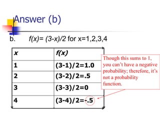
33. Answer:
08
.
1
16
.
1
)
(
16
.
1
2
.
3
4
.
11
)]
(
[
)
(
)
(
4
.
11
)
1
(.
25
)
3
(.
16
)
4
(.
9
)
1
)(.
4
(
)
1
)(.
1
(
)
(
)
(
2
2
2
5
1
2
2
=
=
=
−
=
−
=
=
+
+
+
+
=
=
=
x
stddev
x
E
x
E
x
Var
x
p
x
x
E
i
i
i
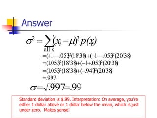
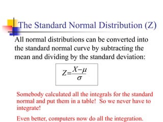
Interpretation: On an average night, we expect Rohan to
awaken 3 times, plus or minus 1.08. This gives you a feel for
what would be considered an unusual night!
x2 1 4 9 16 25
P(x) .1 .1 .4 .3 .1

34. continuous
probability(Gaussian)
distributions:
The normal and standard normal

35. The Normal Distribution
X
f(X)


Changing μ shifts the
distribution left or right.
Changing σ increases or
decreases the spread.

36. The Normal Distribution:
as mathematical function
(pdf)
2
)
(
2
1
2
1
)
( 



−
−

=
x
e
x
f
Note constants:
=3.14159
e=2.71828
This is a bell shaped
curve with different
centers and spreads
depending on  and 

37. The Normal PDF
1
2
1 2
)
(
2
1
=


+

−
−
−
dx
e
x




It’s a probability function, so no matter what the values
of  and , must integrate to 1!

38. Normal distribution is defined
by its mean and standard dev.
E(X)= =
Var(X)=2 =
Standard Deviation(X)=
dx
e
x
x

+

−
−
−

2
)
(
2
1
2
1 



2
)
(
2
1
2
)
2
1
(
2





−


+

−
−
−
dx
e
x
x

39. **The beauty of the normal curve:
No matter what  and  are, the area between - and
+ is about 68%; the area between -2 and +2 is
about 95%; and the area between -3 and +3 is
about 99.7%. Almost all values fall within 3 standard
deviations.

40. 68-95-99.7 Rule
68% of
the data
95% of the data
99.7% of the data

41. 68-95-99.7 Rule
in Math terms…
997
.
2
1
95
.
2
1
68
.
2
1
3
3
)
(
2
1
2
2
)
(
2
1
)
(
2
1
2
2
2
=
•
=
•
=
•



+
−
−
−
+
−
−
−
+
−
−
−
























dx
e
dx
e
dx
e
x
x
x

42. How good is rule for real data?
Check some example data:
The mean of the weight of the women = 127.8
The standard deviation (SD) = 15.5

43. 80 90 100 110 120 130 140 150 160
0
5
10
15
20
25
P
e
r
c
e
n
t
POUNDS
127.8 143.3
112.3
68% of 120 = .68x120 = ~ 82 runners
In fact, 79 runners fall within 1-SD (15.5 lbs) of the mean.

44. 80 90 100 110 120 130 140 150 160
0
5
10
15
20
25
P
e
r
c
e
n
t
POUNDS
127.8
96.8
95% of 120 = .95 x 120 = ~ 114 runners
In fact, 115 runners fall within 2-SD’s of the mean.
158.8

45. 80 90 100 110 120 130 140 150 160
0
5
10
15
20
25
P
e
r
c
e
n
t
POUNDS
127.8
81.3
99.7% of 120 = .997 x 120 = 119.6 runners
In fact, all 120 runners fall within 3-SD’s of the mean.
174.3

46. Example
◼ Suppose SAT scores roughly follows a
normal distribution in the U.S. population of
college-bound students (with range
restricted to 200-800), and the average math
SAT is 500 with a standard deviation of 50,
then:
◼ 68% of students will have scores between 450
and 550
◼ 95% will be between 400 and 600
◼ 99.7% will be between 350 and 650

47. Example
◼ BUT…
◼ What if you wanted to know the math SAT
score corresponding to the 90th percentile
(=90% of students are lower)?
P(X≤Q) = .90 →
90
.
2
)
50
(
1
200
)
50
500
(
2
1 2
=
•

−
−
Q x
dx
e


48. The Standard Normal (Z):
“Universal Currency”
The formula for the standardized normal
probability density function is
2
2 )
(
2
1
)
1
0
(
2
1
2
1
2
)
1
(
1
)
(
Z
Z
e
e
Z
p
−
−
−

=

=



49. The Standard Normal Distribution (Z)
All normal distributions can be converted into
the standard normal curve by subtracting the
mean and dividing by the standard deviation:


−
= X
Z
Somebody calculated all the integrals for the standard
normal and put them in a table! So we never have to
integrate!
Even better, computers now do all the integration.

50. Comparing X and Z units
Z
100
2.0
0
200 X ( = 100,  =
50)
( = 0,  =
1)

51. Example
◼ For example: What’s the probability of getting a math SAT
score of 575 or less, =500 and =50?
5
.
1
50
500
575 =
−
=
Z
⚫i.e., A score of 575 is 1.5 standard deviations above the mean

 
−
−
−
−

⎯
→
⎯

=


5
.
1
2
1
575
200
)
50
500
(
2
1 2
2
2
1
2
)
50
(
1
)
575
( dz
e
dx
e
X
P
Z
x


But to look up Z= 1.5 in standard normal chart (or enter
into SAS)→ no problem! = .9332

52. Answer
a. What is the chance of obtaining a birth
weight of 141 oz or heavier when
sampling birth records at random?
46
.
2
13
109
141 =
−
=
Z
From the chart or SAS → Z of 2.46 corresponds to a right tail (greater
than) area of: P(Z≥2.46) = 1-(.9931)= .0069 or .69 %

53. Answer
b. What is the chance of obtaining a birth
weight of 120 or lighter?
From the chart or SAS → Z of .85 corresponds to a left tail area of:
P(Z≤.85) = .8023= 80.23%
85
.
13
109
120 =
−
=
Z

54. Looking up probabilities in the
standard normal table
What is the area
to the left of
Z=1.51 in a
standard normal
curve?
Z=1.51
Z=1.51
Area is
93.45%