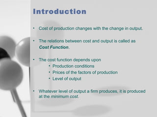
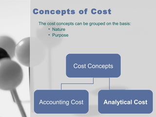
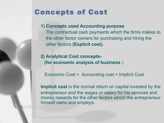
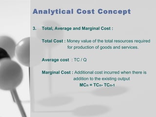
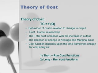
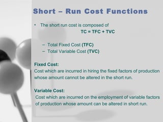
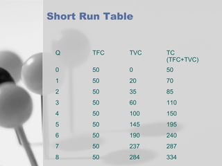
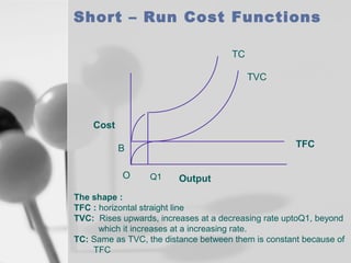
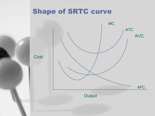
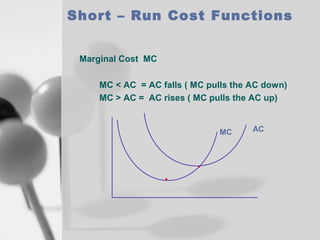
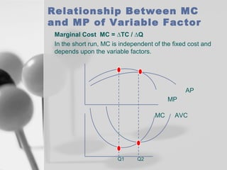
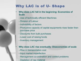
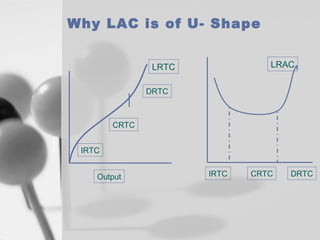
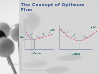
This document discusses cost concepts from an accounting and analytical perspective. It defines different types of costs such as fixed, variable, total, average, and marginal cost. It explains the relationship between these costs and how they change with varying levels of output in the short-run and long-run. The short-run cost curves are U-shaped while the long-run average cost curve is U-shaped, reflecting economies and diseconomies of scale. Other concepts covered include opportunity cost, sunk cost, learning curves, and economies of scope.

1. Cost
Concepts

2. Introduction
• Cost of production changes with the change in output.
• The relations between cost and output is called as
Cost Function.
• The cost function depends upon
• Production conditions
• Prices of the factors of production
• Level of output
• Whatever level of output a firm produces, it is produced
at the minimum cost.

3. Concepts of Cost
The cost concepts can be grouped on the basis:
• Nature
• Purpose
Cost Concepts
Accounting Cost
Analytical Cost

4. Concepts of Cost
1) Concepts used Accounting purpose
The contractual cash payments which the firms makes to
the other factor owners for purchasing and hiring the
other factors (Explicit cost).
2) Analytical Cost concepts(for economic analysis of business )
Economic Cost = Accounting cost + Implicit Cost
Implicit cost is the normal return on capital invested by the
entrepreneur and the wages or salary for his services and
money rewards for the other factors which the entrepreneur
himself owns and employs

5. Concepts of Cost
A firm will earn Economic profits only when its making
revenue to excess of the total of accounting and implicit
cost.
Economic profit = Total revenue – Economic cost

6. Accounting Cost Concepts
1.
Actual cost ( Outlay or Acquisition cost:
The cost that the firm incurs while producing or acquiring a
goods or services. ( cost of raw material, labour, rent…).
They are recorded in the book of accounts
2.
Opportunity Cost:
The return of the second best use of the firm resources
which the firm forgoes in order to avail of the return form
the best use of the resources.
It is an example of implicit cost.
3.
Sunk cost:
The cost which are not altered by change in quantity and
cannot be recovered ( depreciation). They are part of
outlay cost.

7. Accounting Cost Concepts
4.
Business cost and Full cost
Business Cost includes all the expenses which are
incurred to carry out a business.
Full Cost is equal to business cost plus opportunity cost
and normal profit.
5.
Explicit Cost and Implicit cost (Imputed):
Explicit Cost are those which are actually paid by the firm.
Implicit are theoretical cost and go unrecognised by the
firm
Opportunity cost is a part of implicit cost

8. Analytical Cost Concept
1.
Fixed Cost:
Cost which are fixed in volume and do not vary for a
certain level of output
Cost of managerial and administrative staff, depreciation
of machinery, building and fixed assets, maintenance of
land
2.
Variable Cost:
Vary with the variation of total output.
Cost of raw material, cost of direct labour, running
expenses of fixed capital such as fuel, repairs , routine
maintenance

9. Analytical Cost Concept
3.
Total, Average and Marginal Cost :
Total Cost : Money value of the total resources required
for production of goods and services.
Average cost : TC / Q
Marginal Cost : Additional cost incurred when there is
addition to the existing output
MCn = TCn- TCn-1

10. Theory of Cost
Theory of Cost:
TC = f (Q)
–
–
–
–
–
Behaviour of cost in relation to change in output
Cost : Output relationship
The Total cost increases with the increase in output.
The direction of change in Average and Marginal Cost
Cost function depends upon the time framework chosen
for cost analysis:
1) Short – Run Cost Functions
2) Long – Run cost functions

11. Short – Run Cost Functions
•
The short run cost is composed of
TC = TFC + TVC
– Total Fixed Cost (TFC)
– Total Variable Cost (TVC)
Fixed Cost:
Cost which are incurred in hiring the fixed factors of production
whose amount cannot be altered in the short run.
Variable Cost:
Cost which are incurred on the employment of variable factors
of production whose amount can be altered in short run.

12. Short Run Table
Q
TFC
TVC
TC
(TFC+TVC)
0
50
0
50
1
50
20
70
2
50
35
85
3
50
60
110
4
50
100
150
5
50
145
195
6
50
190
240
7
50
237
287
8
50
284
334

13. Short – Run Cost Functions
TC
TVC
Cost
TFC
B
O
Q1
Output
The shape :
TFC : horizontal straight line
TVC: Rises upwards, increases at a decreasing rate uptoQ1, beyond
which it increases at a increasing rate.
TC: Same as TVC, the distance between them is constant because of
TFC

14. Short – Run Cost Functions
AFC: TFC / Q
It falls steadily as output increases. It slopes downwards,
as with increase in output TFC spreads over more units,
as output becomes large, AFC approaches zero.
AVC: TVC / Q
It falls with increase in output (increasing return), but
beyond a normal capacity output, AVC will rise steeply –
diminishing returns.
ATC: TC / Q
ATC curve depends upon the behaviour of AFC and AVC.
Beginning both AVC and AFC falls so ATC also falls.
AVC curve starts rising, but AFC falls, so ATC also falls
With the increase in output, a sharp rise in AVC leads to
rise of ATC.

15. Shape of SRTC curve
MC
ATC
AVC
Cost
AFC
Output

16. Shape of SRTC curve
•
•
•
•
The shape of AC curve depend upon AVC and AFC
In the beginning both AFC and AVC falls, so AC falls
AVC rising and AFC falling, AC still falls
But as output increases, a sharp rise AVC offset the fall
of AFC and AC start to rise

17. Short – Run Cost Functions
Marginal Cost MC
MC < AC = AC falls ( MC pulls the AC down)
MC > AC = AC rises ( MC pulls the AC up)
MC
AC

18. Relationship Between MC
and MP of Variable Factor
Marginal Cost MC = ∆TC / ∆Q
In the short run, MC is independent of the fixed cost and
depends upon the variable factors.
AP
MP
MC
Q1
Q2
AVC

19. Relationship Between
MC and MP of Variable
Factor
•
The behaviour of Marginal Product (MP) determines the
shape of MC.
•
The MC is an inverse of MP, with maximum of MP
corresponding to minimum of MC.
•
MC is the transformation of MP from physical term to
money term.

20. Long – Run Cost Functions
•
A firm can vary all its input
•
The entrepreneur has before him number of alternative plant
sizes and levels of output.
•
In short run the size of the plant ( capital equipment,
machinery, land…) are fixed.
•
In long run the firm can move from one plant to another plant
•
The LRAC is the least possible average cost production of
producing any given level of output when all the inputs are
variable.

21. Derivation of Long Run Average
Cost Curve
SAC1
H
G
Average
cost
J
SAC2
R
L
K
A
B
C
Output
D
SAC3

22. • In long run firm can vary all its input.
• The firm moves from one plant to larger plant if it has to
increase its output.
• The long run average cost of production is the least
possible average cost of producing any given level of output
when all the inputs are variable.
• The short run average cost curves are called as Plant
curves.
• Suppose there are only three technically possible size of
plant.
• The firm can choose among the three possible sizes of
plant
• Upto OB amount of output, the firm will operate on the
SAC1, though it could produce on SAC2.
• For OA output . It will cost AL per unit cost on SAC1 curve
but it will cost AH if on SAC2. (AL < AH).
• If the firm plans to produce larger output than OB then it has
to move to a bigger plant size.
• Thus OC if produced on SAC2 cost CK per unit which is
lower than CJ when produced on SAC1.
• If the firm produce output between OB and OD it will
employ the plant corresponding to SAC2.

23. Long-Run Cost Curve
LAC
F
AC
G
K
M N V
Q
Output

24. Long – Run Cost Functions
•
The LAC is the locus of all the tangency points with the
short run average cost curve.
•
The long curve is also called as Envelope curve.
•
LAC is not tangent to the minimum point of SAC.
•
LRAC is called the planning curve: as the firm plans
to produce any output in the long run by choosing a
plant on the LRAC corresponding to the given output.
•
Point G lies on the falling portion of SAC2, the firm is
using the given plant below its full capacity. Point F is
the minimum point

25. Why LAC is of U- Shape
•
Why does LAC fall in the beginning: Economies of
Scale
- Use of technically efficient Machines
- Division of Labour
- Indivisibility of factors
- Productive capacity of capital equipments rises faster then
purchase price
- Discounts from bulk purchases
- Lower cost of raising funds
- Inventory management
•
Why does LAC rise eventually: Diseconomies of scale
- Rise in transportation cost
- Input market imperfection
- Management co-ordination and control problems
- Depletion of raw material

26. Why LAC is of U- Shape
LRAC
LRTC
DRTC
CRTC
IRTC
Output
IRTC
CRTC
DRTC

27. The Concept of Optimum
Firm
•
The best or the ideal size of the firm
•
The optimum firm is the one which operates on the scale at
which, in the existing condition of techniques and organising
ability has the lowest average cost of production.
•
The optimum size of the firm varies a great deal in different
industries.
– In some industries the minimum point of the long run
average cost curve reaches at a comparatively small
output ( agriculture, wholesale, retail…)
– Optimum size in steel, automobile, heavy industries is
very large and the minimum point is reached at a very
large output.

28. The Concept of Optimum
Firm
LAC
LAC
AC
Output
Output

29. LAC as a Decision making Tool
•
Which plant size to use?
The potential for using a plant of greater capacity is
considerable
- Lowers the AC and MC
But it depends upon the actual forecast of potential demand
As the forecast helps in estimating the production capacity
Incurrence of unnecessary cost by producing at another
plant size
Co-ordination between Production plans and marketing
forecast

30. Long – Run Cost Functions
Capacity
Level
TP
LRTC
MC
LRAC
A
10,000
50,000
5
5
B
20,000
90,000
4
4
C
30,000
120,000
3
4
D
40,000
150,000
3
3.75
E
50,000
200,000
5
4
F
60,000
2,60,000
6
4.33

31. The Learning Curve
•
•
•
•
It is line showing the relationship between labour cost and
additional unit of output.
It’s a downward slope indicates that additional cost per unit
declines as the level of output increases because workers
improve with practice.
Learning is the cumulative through time and enhances the
efficiency, accuracy and productivity.
The more the organisation learns
greater will be productivity.
Cost
Per unit
Output

32. The Learning Curve
• Reasons for fall in average cost:
– Job familiarisation and reduced time to instruct
– Improved operating processes, machine speeds
and feeds
– Improvements in machine and tooling
– Larger manufacturing lots and reducing set up
time
– Better co-ordination and managerial control
Thus learning curve describes the reduction in cost
per unit of Output as a firms cumulative output over
successive time periods increases, while output per
period may remain the same.

33. Economies of Scope
Cost effective for a single firm to produce more than one
product than for separate firms to produce an equal
quantity of output of the same product.
1)
2)
In case of a firm produces several products: common
production facilities and inputs
Production of one good results in by-products that can also
be sold by producers.

34. Economies of Scope
Degree of economies of scope =
TC (Q1) + TC (Q2) – TC (Q1 + Q2)
TC (Q1 + Q2)
TC (Q1) = Total cost of production Q1 units of good 1
TC (Q2) = Total cost of production Q2 units of good 2
TC (Q1 + Q2) = Total cost of producing goods 1 and 2 jointly
•
If Degree of Economies of Scope
– Positive: Economies of Scope exist. Producing goods
jointly is cheaper
– Negative: Producing goods separately is cheaper

35. Case Study – Natasha
Computers
•
Problem of Decision making
– To drop Advanced computers from product line in favour
of old computers with new methods of production.
•
Scenario:
Recession in U.S, Global recession in the computer Industry
Natasha thinks that in order to remain in the competitive
business, the company should adopt new technology in the
production of traditional models, while advanced computers
which have a narrow market at the top, would be most hardhi during recession.
CEO thinks that the best strategy would, therefore be to
produce traditional computers with old as well as new
method of production

36. Case Study – Natasha
Computers
The Pre- recession stage
Fixed cost of Production: Rs 60,00,000
Volume of production:
20,000
Type of
Computers
Price per
Unit ( Rs)
Variable cost Proportion
Per unit
in TP
Traditional
40,000
25,000
50
Advanced
75,000
45,000
50

37. Case Study – Natasha
Computers
The Recession stage
Fixed cost of Production: Rs 6,00,000
Volume of production:
20,000 (Forecasted)
Type of Computers
Price per
Unit ( Rs)
Variable cost Proportion
Per unit
in TP
Traditional by old
method
40,000
25,000
60
Traditional by new
methods of
production
70,000
50,000
40
The logic of producing new and old computers by traditional method is
that
Old is targeted towards mass market which is very price sensitive,
New are quality conscious but within a reasonable price range.