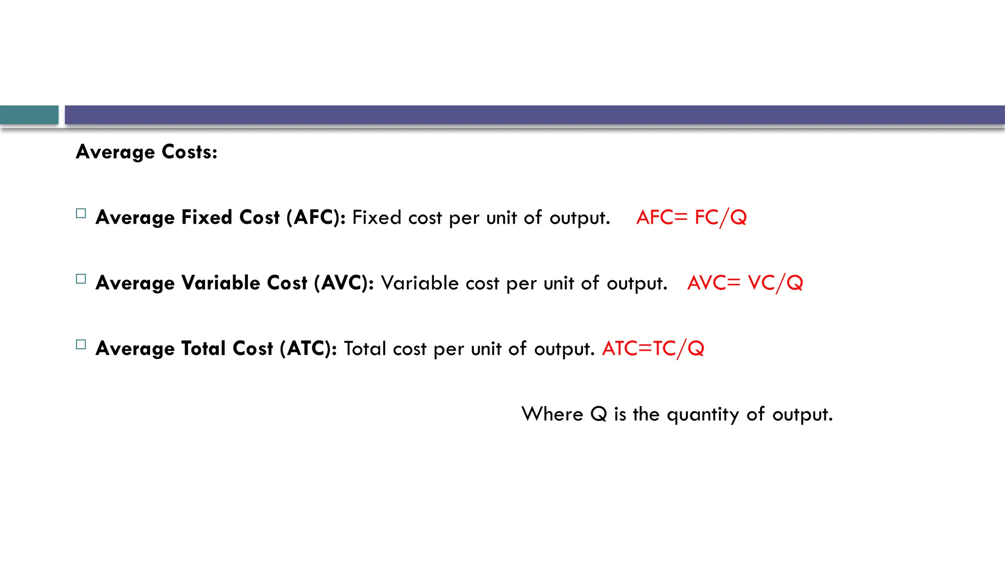
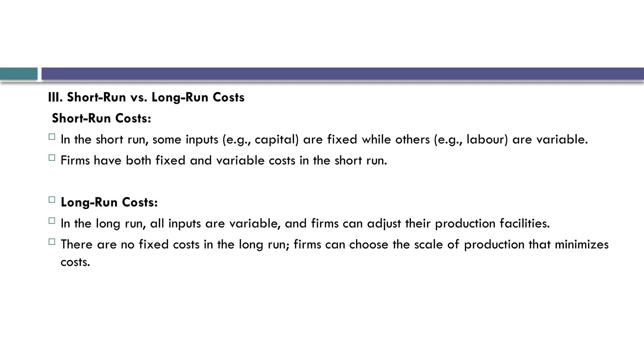
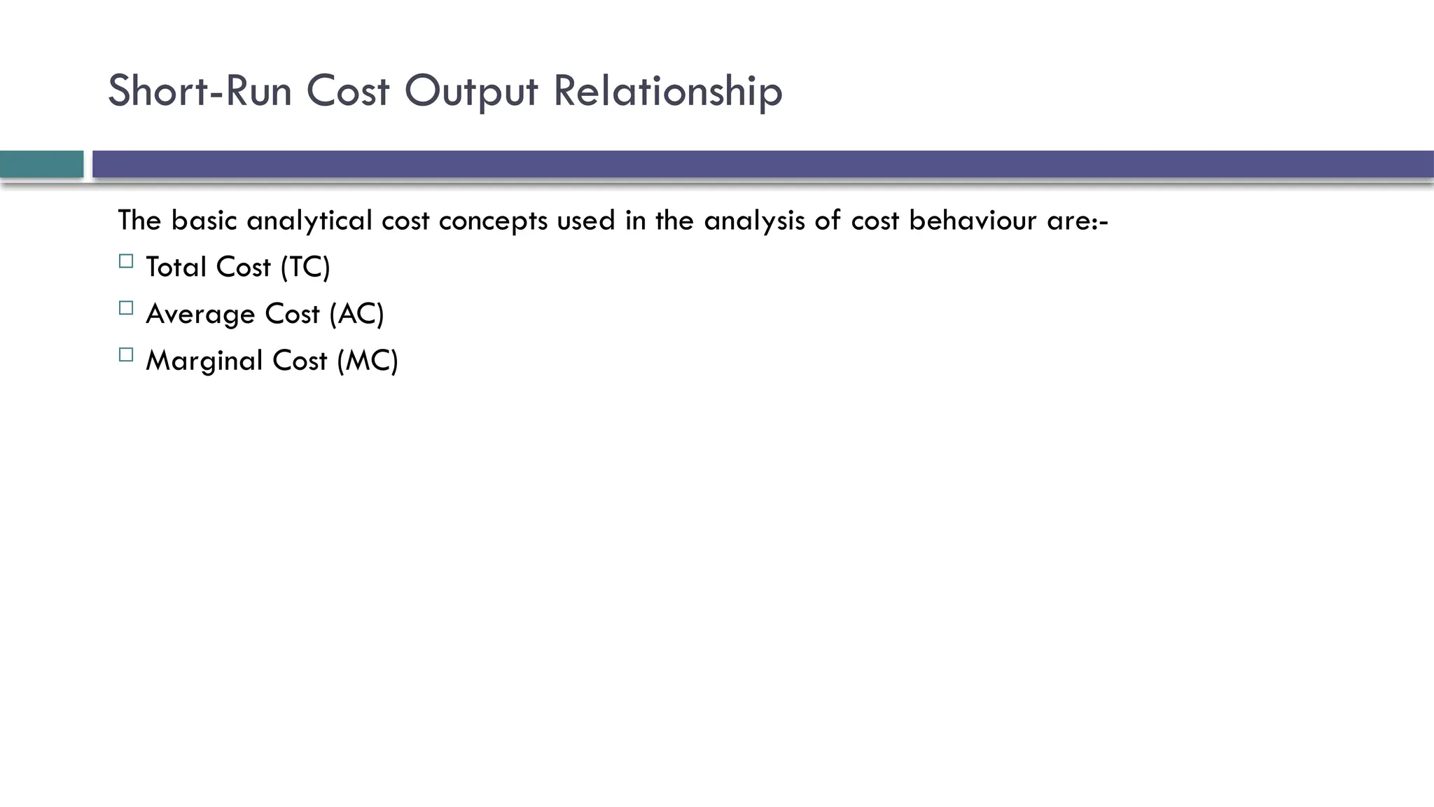
Model Institute of
Engineering & Technology
Course Name-Managerial Economics
Course Code- OEC 701 ( C )
Topic –Cost Analysis
Cost Concepts
 Cost refers to the relationship between production and the expenses incurred to achieve a
certain level of output.
 Cost is the total expenditure incurred in producing a commodity.
 Cost may be defined as the monetary value of all sacrifices made to achieve an objective i.e.
to produce goods and services.
Determinants of cost:
 Price of inputs
 Productivity of inputs
 Technology
 Level of output
Cost Concepts
Cost concepts can be grouped on the basis of their nature and purpose under 2 categories:-
a) Accounting Cost Concepts
b) Analytical Cost Concepts
Analytical Cost Concepts
I. Fixed Costs and Variable Costs:
Fixed Costs
 These are costs that remain constant regardless of the level of output. Examples include rent,
insurance, or salaries of permanent staff.
 Even if the firm produces zero output, fixed costs are still incurred.
Variable Costs (VC):
 Variable costs change directly with the level of output. The more you produce, the higher the
variable costs. Examples include raw materials, energy costs, and wages for hourly workers.
 When output is zero, variable costs are also zero.
II. Total Costs, Average Costs and Marginal Costs:
 Total cost is the sum of fixed and variable costs at each level of output.
 Formula:
TC=FC+VC
Average Costs:
 Average Fixed Cost (AFC): Fixed cost per unit of output. AFC= FC/Q
 Average Variable Cost (AVC): Variable cost per unit of output. AVC= VC/Q
 Average Total Cost (ATC): Total cost per unit of output. ATC=TC​
/Q
Where Q is the quantity of output.
Marginal Cost (MC):
 The additional cost incurred by producing one more unit of output.
 It is important in decision-making as it shows the cost of expanding production.
 Formula:
MC= TC/ Q
Δ Δ
III. Short-Run vs. Long-Run Costs
Short-Run Costs:
 In the short run, some inputs (e.g., capital) are fixed while others (e.g., labour) are variable.
 Firms have both fixed and variable costs in the short run.
 Long-Run Costs:
 In the long run, all inputs are variable, and firms can adjust their production facilities.
 There are no fixed costs in the long run; firms can choose the scale of production that minimizes
costs.
IV. Incremental Costs and Sunk Costs
Incremental Costs
 Incremental costs are the additional costs that a business incurs when it makes a decision to
increase production or implement a change.
 These costs arise due to an increase in production, expansion, or other activities.
Sunk Costs
 Sunk costs are costs that have already been incurred and cannot be recovered, regardless of
future actions or decisions.
Accounting Cost Concepts
I. Opportunity Cost and Actual Cost:
Opportunity Cost
 Opportunity cost is the return expected from the second best use of resources foregone due to
the scarcity of resources.
 It plays a significant role in cost analysis as firms must consider the potential benefits lost when
choosing one option over another.
 Also called as alternative cost.
Actual Cost
 It is all paid out costs of the business firms to take the advantage of best opportunity available
to them.
II. Implicit or Explicit costs
Explicit costs
 It refers to the money expended to buy or hire resources from outside the organization for the
process of production.
Implicit cost
 Implicit cost refers to the cost of use of the self owned resources of organization that are used
in production.
 Implicit costs are not taken into account while calculating the loss or profit of the business.
III. Out of Pocket and Book Costs
Out of Pocket Costs
 The items of expenditure that involve cash payments or cash transfers , both recurring and non
recurring , are known as out-of-pocket costs.
Book Costs
 There are certain actual business costs that do not involve cash payments , but a provision is
therefore made in the books of account and they are taken into account while finalizing the
profit and loss accounts.
Short-Run Cost Output Relationship
The basic analytical cost concepts used in the analysis of cost behaviour are:-
 Total Cost (TC)
 Average Cost (AC)
 Marginal Cost (MC)
 Total Cost is defined as the actual cost that are incurred to produce a given quantity of output.
 The Short run TC is composed of two major elements:
i) Total Fixed Cost (TFC)
ii) Total Variable Cost (TVC)
That is in short run,
TC=TFC+TVC
 Since TFC (i.e. cost of plant , and building etc.,) remains fixed in the short run, where as TVC
(the labour cost) varies with the variation in the output.
 For a given quantity of output (Q), the average cost (AC), average fixed cost (AFC) and
average variable cost (AVC) can be defined as:-
 Marginal Cost (MC) is defined as change in the total cost due to the change in the total output
by one unit, i.e.,
MC=∆TC/ ∆Q= (TCn-TCn-1)/(Qn-Qn-1)
where, (Qn-Qn-1) =1
 It may be added here that since ∆TC= ∆TFC+ ∆TVC and, in the short run, ∆TFC=0, therefore,
∆TC= ∆TVC.
Therefore under the marginality concept , where ∆Q=1; MC= ∆TVC.
Short-Run Cost Functions
 Cost Function: It represent the relationship between the level of output and the cost of
production.
 The short-run cost function specifically refers to the costs incurred by a firm in the short run,
where at least one factor of production is fixed.
 Three concepts of total cost in the short run must be considered: total fixed cost (TFC), total
variable cost (TVC), and total cost (TC).
 Total fixed costs are the total costs per period of time incurred by the firm for fixed inputs.
Since the amount of the fixed inputs is fixed, the total fixed cost will be the same regardless of
the firm’s output rate.
 Total variable costs are the total costs incurred by the firm for variable inputs
A Firm’s Short Run Costs (in Rs.)
 Since total fixed costs are constant, the total fixed cost curve is simply a horizontal line at 100.
 And because total cost is the sum of total variable costs and total fixed costs, the total cost
curve has the same shape as the total variable cost curve but lies above it by a vertical
distance of Rs.100
 Corresponding to our discussion above we can define the following for the short run:
TC = TFC + TVC where,
TC = total cost ; TFC = total fixed costs ; TVC = total variable costs
Average cost
 There are three average cost concepts corresponding to the three total cost concepts. These
are average fixed cost (AFC), average variable cost (AVC), and average total cost (ATC).
 Average fixed cost is the total fixed cost divided by output.
 Average fixed cost declines as output (Q) increases.
 Thus, we can write average fixed cost as: AFC = TFC/Q
 Average Variable Costs is the total variable cost divided by output.
 In average variable cost curve, output increases resulting in decrease in average variable cost,
but beyond a point, they result in higher average variable cost.
 AVC =TVC/Q; where, Q = Output TVC = total variable costs AVC = average variable costs
 Since ATC is sum of the AFC and AVC, ATC curve always exceeds AVC curve.
 Also, since AFC falls as output increases, AVC and ATC get closer as output rises.
 Marginal Cost (MC) is the addition to either total cost or total variable cost resulting from the
addition of one unit of output. Thus, MC = ∆TC/Q;
where, MC = marginal cost;
Q = change in output
Δ
TC = change in total cost due to change in output
Δ
TVC = change in total variable cost due to change in output
Δ
 The MC cuts both AVC and ATC at their minimum.
 When both the MC and AVC are falling, AVC will fall at a slower rate.
 When both the MC and AVC are rising, MC will rise at a faster rate. As a result, MC will
attain its minimum before the AVC.
Cost-Output relationship in the Long Run
 In the long run, all costs are variable, meaning that a firm can adjust its inputs and production
capacity. This allows for more flexibility in the cost-output relationship compared to the short
run.
 The long run cost curve is also called planning curve because it helps the firm in future decision-
making process.
 The long run cost output relationship can be shown with the help of a long run cost curve. The
long run average cost curve (LRAC) is derived from short run average cost curves (SRAC)
 Suppose that at a particular time , a firm operates under average total cost curve U2 and
produces OM.
 Now it is desired to produce ON.
 If the firm continues under old scale, its average cost will be NT . If the scale of the firm will be
altered, the new cost curve would be U3 .
 The average cost of producing will ON would then be NA. NA is less than NT.
 So new scale is preferable to the old one and adopted.
 In the long run the average cost of producing ON output is NA.
 To draw long run cost curves , number of
short run average cost curves(SAC),each
representing a particular scale or size of
the plant are needed.
 Long run cost would be tangential to the
entire family of SAC curves.
 The LAC curve is tangential to various SAC
Curves . It is said to envelope them and is
often called as the “Envelope Curve”.
Estimating Cost Functions
Estimating cost functions involves identifying the relationship between costs and production levels.
Here are methods used to estimate both short-run and long-run cost functions:
1. Historical Data Analysis:
 Collecting and analysing historical cost data related to production levels helps identify patterns and
relationships.
 Cost data can be classified into fixed and variable components, providing insights into cost behaviour.
2. Engineering Cost Analysis:
 This method involves a detailed examination of the production process to determine input requirements,
labour, and material costs.
 Engineers analyse how changes in output levels impact total costs based on resource utilization.
3. Statistical Methods:
 Regression Analysis: Using statistical techniques to fit a cost function model to historical data.
 Linear Regression can be employed to estimate the cost function as:
TC=a + bQ
where a is the fixed cost, b is the variable cost per unit, and Q is the quantity produced.
 Multiple Regression Analysis: Useful for estimating cost functions that depend on several
factors, such as labour hours, material costs, and production volume.
4. Cost-Volume-Profit (CVP) Analysis:
 This method evaluates how changes in cost and volume affect a company’s operating income
and net income. It helps in estimating both short-run and long-run costs.
5. Activity-Based Costing (ABC):This method assigns costs to products based on the resources
consumed in production. It provides a more accurate representation of the cost structure,
particularly in complex production environments.

Cost analysis is the name of the ppt and

  • 1.
    Model Institute of Engineering& Technology Course Name-Managerial Economics Course Code- OEC 701 ( C ) Topic –Cost Analysis
  • 2.
    Cost Concepts  Costrefers to the relationship between production and the expenses incurred to achieve a certain level of output.  Cost is the total expenditure incurred in producing a commodity.  Cost may be defined as the monetary value of all sacrifices made to achieve an objective i.e. to produce goods and services.
  • 3.
    Determinants of cost: Price of inputs  Productivity of inputs  Technology  Level of output
  • 4.
    Cost Concepts Cost conceptscan be grouped on the basis of their nature and purpose under 2 categories:- a) Accounting Cost Concepts b) Analytical Cost Concepts
  • 5.
    Analytical Cost Concepts I.Fixed Costs and Variable Costs: Fixed Costs  These are costs that remain constant regardless of the level of output. Examples include rent, insurance, or salaries of permanent staff.  Even if the firm produces zero output, fixed costs are still incurred. Variable Costs (VC):  Variable costs change directly with the level of output. The more you produce, the higher the variable costs. Examples include raw materials, energy costs, and wages for hourly workers.  When output is zero, variable costs are also zero.
  • 6.
    II. Total Costs,Average Costs and Marginal Costs:  Total cost is the sum of fixed and variable costs at each level of output.  Formula: TC=FC+VC
  • 7.
    Average Costs:  AverageFixed Cost (AFC): Fixed cost per unit of output. AFC= FC/Q  Average Variable Cost (AVC): Variable cost per unit of output. AVC= VC/Q  Average Total Cost (ATC): Total cost per unit of output. ATC=TC​ /Q Where Q is the quantity of output.
  • 8.
    Marginal Cost (MC): The additional cost incurred by producing one more unit of output.  It is important in decision-making as it shows the cost of expanding production.  Formula: MC= TC/ Q Δ Δ
  • 9.
    III. Short-Run vs.Long-Run Costs Short-Run Costs:  In the short run, some inputs (e.g., capital) are fixed while others (e.g., labour) are variable.  Firms have both fixed and variable costs in the short run.  Long-Run Costs:  In the long run, all inputs are variable, and firms can adjust their production facilities.  There are no fixed costs in the long run; firms can choose the scale of production that minimizes costs.
  • 10.
    IV. Incremental Costsand Sunk Costs Incremental Costs  Incremental costs are the additional costs that a business incurs when it makes a decision to increase production or implement a change.  These costs arise due to an increase in production, expansion, or other activities. Sunk Costs  Sunk costs are costs that have already been incurred and cannot be recovered, regardless of future actions or decisions.
  • 11.
    Accounting Cost Concepts I.Opportunity Cost and Actual Cost: Opportunity Cost  Opportunity cost is the return expected from the second best use of resources foregone due to the scarcity of resources.  It plays a significant role in cost analysis as firms must consider the potential benefits lost when choosing one option over another.  Also called as alternative cost. Actual Cost  It is all paid out costs of the business firms to take the advantage of best opportunity available to them.
  • 12.
    II. Implicit orExplicit costs Explicit costs  It refers to the money expended to buy or hire resources from outside the organization for the process of production. Implicit cost  Implicit cost refers to the cost of use of the self owned resources of organization that are used in production.  Implicit costs are not taken into account while calculating the loss or profit of the business.
  • 13.
    III. Out ofPocket and Book Costs Out of Pocket Costs  The items of expenditure that involve cash payments or cash transfers , both recurring and non recurring , are known as out-of-pocket costs. Book Costs  There are certain actual business costs that do not involve cash payments , but a provision is therefore made in the books of account and they are taken into account while finalizing the profit and loss accounts.
  • 14.
    Short-Run Cost OutputRelationship The basic analytical cost concepts used in the analysis of cost behaviour are:-  Total Cost (TC)  Average Cost (AC)  Marginal Cost (MC)
  • 15.
     Total Costis defined as the actual cost that are incurred to produce a given quantity of output.  The Short run TC is composed of two major elements: i) Total Fixed Cost (TFC) ii) Total Variable Cost (TVC) That is in short run, TC=TFC+TVC  Since TFC (i.e. cost of plant , and building etc.,) remains fixed in the short run, where as TVC (the labour cost) varies with the variation in the output.
  • 16.
     For agiven quantity of output (Q), the average cost (AC), average fixed cost (AFC) and average variable cost (AVC) can be defined as:-
  • 17.
     Marginal Cost(MC) is defined as change in the total cost due to the change in the total output by one unit, i.e., MC=∆TC/ ∆Q= (TCn-TCn-1)/(Qn-Qn-1) where, (Qn-Qn-1) =1  It may be added here that since ∆TC= ∆TFC+ ∆TVC and, in the short run, ∆TFC=0, therefore, ∆TC= ∆TVC. Therefore under the marginality concept , where ∆Q=1; MC= ∆TVC.
  • 18.
    Short-Run Cost Functions Cost Function: It represent the relationship between the level of output and the cost of production.  The short-run cost function specifically refers to the costs incurred by a firm in the short run, where at least one factor of production is fixed.  Three concepts of total cost in the short run must be considered: total fixed cost (TFC), total variable cost (TVC), and total cost (TC).  Total fixed costs are the total costs per period of time incurred by the firm for fixed inputs. Since the amount of the fixed inputs is fixed, the total fixed cost will be the same regardless of the firm’s output rate.  Total variable costs are the total costs incurred by the firm for variable inputs
  • 19.
    A Firm’s ShortRun Costs (in Rs.)
  • 21.
     Since totalfixed costs are constant, the total fixed cost curve is simply a horizontal line at 100.  And because total cost is the sum of total variable costs and total fixed costs, the total cost curve has the same shape as the total variable cost curve but lies above it by a vertical distance of Rs.100  Corresponding to our discussion above we can define the following for the short run: TC = TFC + TVC where, TC = total cost ; TFC = total fixed costs ; TVC = total variable costs
  • 22.
    Average cost  Thereare three average cost concepts corresponding to the three total cost concepts. These are average fixed cost (AFC), average variable cost (AVC), and average total cost (ATC).  Average fixed cost is the total fixed cost divided by output.  Average fixed cost declines as output (Q) increases.  Thus, we can write average fixed cost as: AFC = TFC/Q  Average Variable Costs is the total variable cost divided by output.  In average variable cost curve, output increases resulting in decrease in average variable cost, but beyond a point, they result in higher average variable cost.  AVC =TVC/Q; where, Q = Output TVC = total variable costs AVC = average variable costs
  • 24.
     Since ATCis sum of the AFC and AVC, ATC curve always exceeds AVC curve.  Also, since AFC falls as output increases, AVC and ATC get closer as output rises.  Marginal Cost (MC) is the addition to either total cost or total variable cost resulting from the addition of one unit of output. Thus, MC = ∆TC/Q; where, MC = marginal cost; Q = change in output Δ TC = change in total cost due to change in output Δ TVC = change in total variable cost due to change in output Δ
  • 25.
     The MCcuts both AVC and ATC at their minimum.  When both the MC and AVC are falling, AVC will fall at a slower rate.  When both the MC and AVC are rising, MC will rise at a faster rate. As a result, MC will attain its minimum before the AVC.
  • 26.
    Cost-Output relationship inthe Long Run  In the long run, all costs are variable, meaning that a firm can adjust its inputs and production capacity. This allows for more flexibility in the cost-output relationship compared to the short run.  The long run cost curve is also called planning curve because it helps the firm in future decision- making process.  The long run cost output relationship can be shown with the help of a long run cost curve. The long run average cost curve (LRAC) is derived from short run average cost curves (SRAC)
  • 28.
     Suppose thatat a particular time , a firm operates under average total cost curve U2 and produces OM.  Now it is desired to produce ON.  If the firm continues under old scale, its average cost will be NT . If the scale of the firm will be altered, the new cost curve would be U3 .  The average cost of producing will ON would then be NA. NA is less than NT.  So new scale is preferable to the old one and adopted.  In the long run the average cost of producing ON output is NA.
  • 29.
     To drawlong run cost curves , number of short run average cost curves(SAC),each representing a particular scale or size of the plant are needed.  Long run cost would be tangential to the entire family of SAC curves.  The LAC curve is tangential to various SAC Curves . It is said to envelope them and is often called as the “Envelope Curve”.
  • 30.
    Estimating Cost Functions Estimatingcost functions involves identifying the relationship between costs and production levels. Here are methods used to estimate both short-run and long-run cost functions: 1. Historical Data Analysis:  Collecting and analysing historical cost data related to production levels helps identify patterns and relationships.  Cost data can be classified into fixed and variable components, providing insights into cost behaviour. 2. Engineering Cost Analysis:  This method involves a detailed examination of the production process to determine input requirements, labour, and material costs.  Engineers analyse how changes in output levels impact total costs based on resource utilization.
  • 31.
    3. Statistical Methods: Regression Analysis: Using statistical techniques to fit a cost function model to historical data.  Linear Regression can be employed to estimate the cost function as: TC=a + bQ where a is the fixed cost, b is the variable cost per unit, and Q is the quantity produced.  Multiple Regression Analysis: Useful for estimating cost functions that depend on several factors, such as labour hours, material costs, and production volume.
  • 32.
    4. Cost-Volume-Profit (CVP)Analysis:  This method evaluates how changes in cost and volume affect a company’s operating income and net income. It helps in estimating both short-run and long-run costs. 5. Activity-Based Costing (ABC):This method assigns costs to products based on the resources consumed in production. It provides a more accurate representation of the cost structure, particularly in complex production environments.

Editor's Notes

  • #1 Presentation slide for courses, classes, lectures et al.