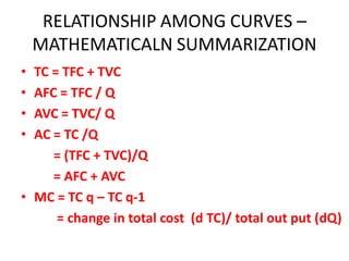
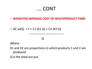
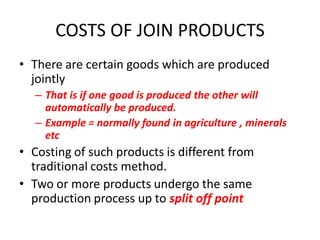
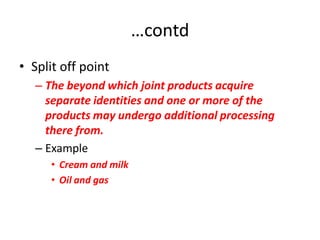
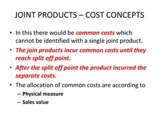
The document discusses various concepts related to cost. It defines cost as a sacrifice or foregone opportunity measured in monetary terms. It then discusses different types of costs such as fixed costs, variable costs, sunk costs, explicit costs, implicit costs, and others. It also discusses cost determination factors and different cost curves and functions in the short run and long run, including total cost, average cost, and marginal cost curves. Finally, it discusses costs for multi-product firms and joint products.

1. COST
(COST MEANS SACRIFICE)

2. MEANING - COST
“ Cost is a sacrifice or foregoing that has
occurred or has potential to occur in future,
measured in monetary terms”
• Cost results in current or future decrease in
cash or other assets or a current or future
increase in liability

3. DETERMINANTS OF COST
• Cost is determined by various factors and each of
these has significant implications for cost
decisions.
• An increase in any of these will affect cost
pattern.
• Important determinant
– Price(uncontrollable –largely determined by external
environment)
– Marginal efficiency and productivity
– Technology
– Level of out put.

4. MATHEMATICAL EXPRESSION- COST
C= F( Q , T , P)
• Where
– C= cost
– Q= out put
– T= technology
– P= price
• Cost are differentiated according to their
purpose , type of product and time.

5. TYPES OF COSTS
• There may be different types of costs incurred
by a firm under different circumstances.
• Cost of a firm may include money or may not
be measurable in money terms.
• Cost is a function of output in economic
theory.
• A managerial economist’s concept of cost
does not necessarily coincide with that of
accountants.

6. TYPES OF COST
• Actual Costs / Acquisition / outlay : It means
the actual expenditure incurred for acquiring
or producing a good or service. These are
generally recorded in the books of accounts.
Eg. Wages paid, cost of materials purchased,
interest paid, etc.
• Opportunity Cost / Alternative Cost: Revenue
forgone by not making the best alternative
use or opportunities.

7. • Imputed Cost / Implicit cost: They are the costs
which are not actually incurred but would have
been incurred in the absence of employment of
self-owned factors. These are unrecognized by
the accounting systems. Eg. Rent of own
building, Salary for Entrepreneur, etc.
• Explicit cost / Paid out costs: Those expenses
which are actually paid by the firm. Appears in
the accounting books.
• Sunk Costs / Non-avoidable / Non escapable:
They are not altered by a change in quantity and
cannot be recovered. All the past expenses are
sunk costs Eg Depreciation, interest, machineries
not in use.

8. • Incremental / Differential cost ( Avoidable,
escapable or Differential): It is the additional
cost due to a change in level or nature of
business activity.
• Out-of-Pocket costs: These are expenses
which are current cash payments to the
outsiders. (All Explicit costs)
• Book Costs: These are business costs which do
not involve any cash payments but for them a
provision is made in the books of account. Eg.
Depreciation, Implicit cost.

9. • Accounting cost / Past Cost: How much
expenditure has already been incurred on a
particular process or on production as such.
• Economic cost / Future cost: Cost relate to
future.
• Direct costs / Traceable / Assignable: These
costs have direct relationship with a unit of
operation.
• Indirect / Non-traceable / Non assignable:
These costs cannot be easily & definitely
traced to a plant or department.

10. • Historical Cost / Original cost: It states the
cost of plant, equipment and materials at the
price paid originally for them.
• Replacement cost: It states the cost that the
firm would have to incur if it wants to replace
or acquire the same assets now.
• Controllable costs: Costs which are capable of
being controlled or regulated.
• Non-Controllable cost: costs which cannot be
subjected to administrative control and
supervision. Eg. Depreciation, Obsolescence.

11. • Private costs: Micro level. Costs incurred by an
individual or a firm for its business activity.
• Social costs: Macro level. Total cost s to the
society on account of production of a good.
• Shutdown Costs: Those costs incurred when
firm temporarily stops it operations.
• Abandonment Costs: Costs incurred when the
firm is retiring altogether.
• Short run costs: a period in which the supply
of at least one of the inputs cannot be
changed by the firm. Inputs are fixed.

12. • Long run costs: Period in which all inputs can
be carried as desired.
• Fixed Cost: Part of total cost of the firm which
does not vary with output.
• Variable cost: Part of total cost that are
directly dependent on the volume of output
or service.
• Total cost: It is money value of the total
resources required for production of goods
and services by the firm. TC = FC + VC

13. • Average cost: It is the cost per unit of output.
– AC = TC / n
– n = number of unit
• Marginal cost: It is the change in total cost
due to unit change in out put
MCn  (TCn  TCn1 )

14. COSTS IN SHORT RUN
• Classification of costs is on the basis of time
– Short run cost
– Long run cost
• The short run is a time period where some
factors of production remain fixed and only
few are variable.
– Fixed inputs – land ,machine and technology
– Variable inputs – labor and raw material

15. Contd…
• Therefore in short run we divide costs in two
broad categories
– Fixed costs
• Costs on fixed inputs
– Variable costs
• Costs on variable inputs

16. TOTAL COSTS FUNCTIONS AND CURVES
FOR SHORT RUN
• As we discussed short run cost have two
components
• Fixed cost
– This cost do not vary with output
– Cost incurred in plant, machinery fitting ,
equipments, land etc.
– Any change in volume of output does not depends
upon fixed cost
– The shape of the TFC(TOTAL FIXED COST) curve is
straight line from origin parallel to quantity axis.

17. GRAPH - TFC
X AXIS – QUANTITY
Y AXIS – COST
TFC

18. • Variable cost
– These are costs that vary with output and are
incurred in getting more and more inputs.
– Variable costs are equal to zero if there is no out
put
– Cost of raw materials , wages are called variable
cost.
– TVC is an inverse S shaped upward sloping curve
starting from origin.

19. GRAPH - TVC
X AXIS – QUANTITY
Y AXIS – COST

20. GRAPH INFERENCE
• The shape of curve determined by law of
variable proportions.
• According to this law as more and more units
of the variable factor are added in production
its productivity goes on increasing.
• This lead to fall in per unit cost in the
beginning. if the variable input is increased
beyond certain level its marginal productivity
starts diminishing.
• So TVC increases at increasing rate.

21. GRAPH – TOTAL COST
TC
TVC
TFC
X AXIS – QUANTITY
TOTAL COST = TFC + TVC
Y AXIS – COST

22. SHORT RUN – AVERAGE AND MARGINAL COST
• AVERAGE COST
– Average cost is cost per unit of out put
– We can derive AFC (average fixed cost) AVC( average
variable cost) and AC (average cost) from total fixed ,
total variable and total costs respectively.
– AFC is fixed cost per unit of output and this is equal to
the ratio of TFC and units of output
• AFC = TFC / NUMBER OF UNITS OF OUT PUT
– AVC is variable cost per unit of out put and this is
equal to the ratio of TVC and units of output
• AVC = TVC / NUMBER OF UNITS OF OUT PUT
– AC is total cost per unit of out put
• AC = TC /NUMBER UNITS OF OUTPUT

23. • MARGINAL COST
– MC is the change in total cost due to unit change
in out put
– Rate of change in total cost.
MCn  (TCn  TCn1 )

24. AVERAGE AND MARGINAL COST CURVES-
SHORT RUN
MC
AC
AVC
AFC
X AXIS – QUANTITY
Y AXIS – COST

25. AVC , AFC AND AC GRAPH -
INFERENCE
• The AVC and AC curve are both U shaped.
– This explained by law of diminishing returns.
– Cost decline when there are increasing
returns(output)
• AC being the sum of AFC and AVC at each
level of output lies above both AFC and AVC
curve.
• Initially AC falls with increase in out put
reaches minimum and then increases.

26. ..contd
• When both AFC and AVC fall AC also falls.
• AVC soon reaches minimum and start rising .
• While AFC continues to fall.
• How ever the rise in AVC compensate falls in
AFC and AVC pulls AC up after reaches a
minimum.

27. MARGINAL COST GRAPH - INFERENCE
• The magnitude of marginal cost is interlinked
with changes in average cost.
• When average cost decline MC lies below AC.
• When average costs are constant the MC passes
through the minimum points of average cost
curves.
• When average cost rise MC curve lies above
them.
• AC and AVC fall MC lies below them
• AC and AVC rise MC lies above them.

28. RELATIONSHIP AMONG CURVES –
MATHEMATICALN SUMMARIZATION
• TC = TFC + TVC
• AFC = TFC / Q
• AVC = TVC/ Q
• AC = TC /Q
= (TFC + TVC)/Q
= AFC + AVC
• MC = TC q – TC q-1
= change in total cost (d TC)/ total out put (dQ)

29. COSTS IN LONG RUN
• All cost are variable in the long run since factors
of production
– Size of plant
– Machinery and technology are all variable.
• The long run cost function is often referred to as
the “planning cost function”
• The long run average cost (LAC) curve is known
as the “ planning curve”
• All the cost are variable only the average cost
curve is relevant to the firm’s decision making
process in the long run.
• Long run cost curve is the composite of many
short run cost curves……*

30. LONG RUN AVERAGE COST (LAC)
• When the plant size and other fixed inputs of
the firm increase in the long run the short run
cost curves shift to the right.
• We consider in the long run the firm operates
with three different plant sizes
– Plant size I , II , III
• It can switch over to a different plant size
depending on cost consideration.

31. …CONTD
• SAC 1 relates to average cost of the firm
when the plant size I.
• When the plant size increases to II the
corresponding SAC 1 curve is SAC 2 and so
on.
• So
– Plant size I – SAC I
– Plant size II – SAC II
– Plant size III – SAC III

32. X AAXIS – QUANTITY
LAC CURVE Y AXIS –AC,MC
MC1 MC2 MC3
SAC1 SAC2 SAC3
plant size I plant size II plant size III
Q0 Q1 Q2

33. GRAPH- INFERENCE
• As out put increases from Qo to Q1 in the short
run the firm can continue to produce along
SAC1, utilizing its installed capacity of plant size I.
• Further ahead at an out put level of Q1 this
capacity is over worked.
• So it would be the cost effective for the firm to
shift to higher plant size say plant size II.
– Thus switching from SAC1 to SAC2
• This shift would lower the average cost of the
firm.
• The same concept is followed for subsequent
output.

34. …contd
• The LAC curve has a scalloping pattern as its
is drawn with three plant sizes only.
• We assumed that the firm operates with only
3 alternative plant sizes.
– But in reality ……………. Multiple such
alternatives.
– So in reality it may have multiple SAC also….
• The LAC function is an envelope of the short
run cost functions and LAC curves envelopes
the SAC curve hence LAC curve is also known
as “ envelope curve”

35. ..contd
• The LAC curve is also known as “planning
curve”
• According to the entire planning horizon in
which the managerial economist can select
the most appropriate plant size , given the
existing (or expected) level of demand for the
product.

36. X AAXIS – QUANTITY
LAC - ENVELOPECURVE Y AXIS –AC,MC
SMC1 SMC2
SAC1 SMC2 SAC3
SAC2
Q0 Q1 Q* Q3

37. LONG RUN MARGINAL COST
• Long run marginal cost (LMC) curve joints the
points on the short run marginal cost (SMC)
curves.

38. X AAXIS – QUANTITY
LMC - CURVE Y AXIS –AC,MC
SMC1 SMC2
C
SAC1 SMC2 SAC3
SAC2
A LMC
B
Q0 Q1 Q* Q3

39. GRAPH INFERENCE
• At out put level of Qo. The relevant long run
marginal cost is Aqo.
• The LMC curve joins the points A,B,C
• According to assuming sufficient demand the
optimum plant size is II.
• So the optimum level of out put is Oq*.
– Where long run and short run marginal cost and
average costs are equal.

40. LAC – DIFFERENT SHAPES
X AAXIS – QUANTITY
Y AXIS –AC

41. LONG RUN TOTAL COST - CURVE
COST LRTC
QUANTITY

42. GRAPH - INFERENCE
• Once we have the long run average cost of
producing an output we can readily derive the
long run total cost of output.
• Since total cost is the quantity of output
times average cost.

43. COST OF A MULTIPRODUCT FIRM
• So far we have assumed that the firm
produces a single good /service.
• How ever in the real business world many
firms produce more than one product.
• A cost of multiproduct firm is differ from costs
of single product.
• In order to ascertain the costs of multiproduct
form we need to first modify some of the cost
concepts.

44. EXAMPLE
• Take multiproduct firm producing 2 goods
– Product 1 and product 2
• For simplicity we assume that the firm uses
the same capital requirements in producing
the above 2 goods.
• So TC of production would be the sum of
fixed cost (TFC) and total variable cost (TVC)-
C1 and C2 of producing both the product
times the quantities of 2 goods be Q1 and Q2
– TC = TFC + C1 Q1 + C2 Q2

45. …. CONT
– WEIGHTED AVERAGE COST OF MULTIPRODUCT FIRM
– AC w(Q) = F + C1 (X1 Q) + C2 (X2 Q)
----------------------------------
Q
Where
X1 and X2 are proportions in which products 1 and 2 are
produced
Q is the total out put.

46. COSTS OF JOIN PRODUCTS
• There are certain goods which are produced
jointly
– That is if one good is produced the other will
automatically be produced.
– Example = normally found in agriculture , minerals
etc
• Costing of such products is different from
traditional costs method.
• Two or more products undergo the same
production process up to split off point

47. …contd
• Split off point
– The beyond which joint products acquire
separate identities and one or more of the
products may undergo additional processing
there from.
– Example
• Cream and milk
• Oil and gas

48. JOINT PRODUCTS – COST CONCEPTS
• In this there would be common costs which
cannot be identified with a single joint product.
• The join products incur common costs until they
reach split off point.
• After the split off point the product incurred the
separate costs.
• The allocation of common costs are according to
– Physical measure
– Sales value

49. LINKAGE BETWEEN COST, REVENUE
AND OUTPUT
• TOTAL REVENUE (TR)
– Total revenue is the total amount of money received
by a firm from goods sold during certain period of
time.
– TR = Q X P
• Q – QUANTITY P – PRICE
• AVERAGE REVENUE (AR)
– Average revenue is the revenue earned per unit of
output sold.
– It is equal to the ratio of TR and out put
– AR = TR / Q
= (Q x P) / Q
– AR = P

50. …CONTD
• MARGINAL REVENUE (MR)
– Marginal revenue is the revenue a firm gains in
producing one additional unit of a commodity
– It is calculated by determining the difference
between the total revenues earned before and
after increase in production
– MRq = TRq - TR q-1
= d TR / d Q

51. TR AND MR - RELATIONSHIP
X AAXIS – QUANTITY
Y AXIS –PRICE ,
REVENUE
MR is slope of TR CURVE
TR
MR

52. GRAPH - INFERENCE
• The graph shows the relationship between total
revenue and marginal revenue.
• TR will be zero when nothing is sold.
• The shape of TR curve is inverted U starts from
origin.
• After it reaches maximum dipping to X axis.
• Rise in total revenue curve is the change in total
revenue with rise in level of output
– So therefore we can say MR is the slope of TR curve

53. MR AND AR – RELATION SHIP
• AR curve can have the following positions
– Straight line
– Convex to the origin X AAXIS – QUANTITY
Y AXIS –MR
– Concave to the origin
PANEL A PANEL B PANEL C
AR AR AR
MR MR MR

54. GRAPH INFERENCE
• PANEL A
– When AR is a straight line MR will be lie midway
to AR
• PANEL B
– When AR is convex to the origin MR will lie less
than midway to AR
• PANEL C
– When AR is concave to the origin MR will lie
more than midway to AR

55. PROFIT MAXIMIZATION
• The profit function shows a range of outputs
at which the firm makes positive profits
• Two types of profits
– Normal profit
• It is amount of return to the firm which must be
earned to keep in that business activity
• It is the part of total cost
– Supernormal profit
• Any thing above normal profit is super normal profit
• It is accounting profit occurs when TR > TC

56. ..CONTD
• A firm maximizes profit at the point where
MR = MC
• Rules of optimization
– The second order condition of profit
maximization requires the slope of MR = slope of
MC

57. BREAK EVEN ANALYSIS
“Break even point is the point where total cost
just equals the total revenue it is the no profit
and no loss point”
• It is also known as cost volume profit analysis
• It is a first step in planning decision

58. APPROACHES IN BREAK EVEN
ANALYSIS
• Graphical method
• Algebraic method
• Contribution margin
• PV ratio
• Margin of safety.

59. GRAPHICAL METHOD
TR
PROFIT
TC
E
VC
FC
X AAXIS – QUANTITY
Y AXIS – COST
REVEUE

60. DRAWING -BREAK EVEN GRAPH
• The break even chart assumes constant AVC for a given
range of output.
• After point E the firm achieve profit.
• The point E is the break even point.
• The gap between the total costs line and revenue line
beyond the break even point represents the level of
profit.
• If the gap is such that TC line is above the TR line the
area represent loss.
• If the TR line is above TC line the area represent profit

61. ALGEBRAIC METHOD
• Let us understand the break even analysis
algebraically
• Let P be the price of a goods
• Q is the quantity produced
• AVC be the average variable cost
• AFC be the average fixed cost
• Let Q* be the break even output, where total
revenue equals total cost.

62. ..contd
• TOTAL REVENUE (TR) = P x Q
• TOTAL COST (TC) = TFC + TVC
= TFC + AVC x Q
• P x Q = TFC + AVC x Q
• (P – AVC) x Q = TFC
Q= TFC/ (P- AVC)

63. CONTRIBUTION MARGIN
• Contribution margin per unit sales is the
difference between price and average variable
cost
– CONTRIBUTION MARGIN = P – AVC
• It represents that portion of the price of the
commodity produced by the firm that can
cover the fixed costs and contribute to profits

64. PV RATIO
• Profit volume (PV) ratio is the ratio of
contribution margin and sales
• It is defined as the ratio of marginal change in
profit and marginal change in sales
• PV RATIO = CONTRIBUTION / SALES
• BEP = FC / PV RATIO
– FC = FIXED COST

65. MARGIN OF SAFETY
• Margin of safety
= planned sales – break even sales

66. LIMITATIONS – BREAK EVEN ANALYSIS
• It does not take into account possible changes
in costs over the time period under
consideration
• It assumes that whatever is produced is sold
• It does not keep any provision for a changes in
selling price.
• It does not allow for changes in market
conditions
• It is difficult to find out BEP in service sector.

67. ECONOMIES OF SCALE
• “Economies” refer to lower costs hence
economies of scale would mean lowering of
costs of production by way of producing in bulk.
• In simple terms economies of scale refers to the
efficiencies associated with large scale of
operations.
• When production increases the average cost per
unit decreases.
• Economies of scale are extremely important in
real world production processes.

68. TYPES OF ECONOMICS OF SCALE
• INTERNAL ECONOMIES OF SCALE
– Cost per unit depends upon the size of the firm
• EXTERNAL ECONOMIES OF SCALE
– Cost per unit depends upon the size of the
industry not the firm.

69. INTERNAL ECONOMIES
• The reason behind the internal economies
– Specialization
• Jobs can be broken down into components/process
• Specialization in particular job
– Greater efficiency of machine
– Managerial economies
• Better supervision, administration, planning & organization
– Financial economies
• Large firms going for large volume of production may able to
raise capital from the market with much less difficulties than
small firm.
– Production in stages
• Houses all the process in production

70. EXTERNAL ECONOMIES
• The reason behind external economies
• As an industry grows in size would create
various economies for existing firms in the
industry
– Technological advancement.
– Easier access to cheaper raw materials.
– Financial institutions in proximity.
– Pool of skilled labors.

71. DISECONOMIES OF SCALE
• It is a reverse of economies of scale.
• It is refers to decreases in productivity when
there are equal increases of all inputs. Assuming
that no inputs is fixed.
• Diseconomies may rise if the size of operations
become un widely by size.
– Coordinating among different work groups and units
may become complex
– Management become less effective and thus
indirectly improve costs