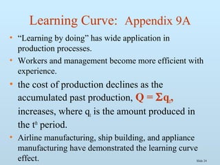
The document discusses various methods for estimating cost functions, including both short run and long run techniques, such as regression analysis and engineering cost approaches. It provides examples of cost estimates for firms like Boeing and utilities, and includes discussions on break-even analysis and the degree of operating leverage. Additionally, it touches on the learning curve effect in production processes.

1. Slide 1
Applications of Cost Theory
Chapter 9
• Estimation of Cost Functions using regressions
» Short run -- various methods including polynomial
functions
» Long run -- various methods including
• Engineering cost techniques
• Survivor techniques
• Break-even analysis and operating leverage
• Risk assessment
• Appendix 9A: The Learning Curve

2. Slide 2
Estimating Costs in the SR
• Typically use TIME SERIES data for a plant or
firm.
• Typically use a functional form that “fits” the
presumed shape.
• For TC, often CUBIC
• For AC, often QUADRATIC
quadratic is U-shaped or arch shaped.
cubic is S-shaped
or backward S-shaped

3. Estimating Short Run Cost Functions
• Example: TIME
SERIES data of total
cost
• Quadratic Total Cost
(to the power of two)
TC = C0 + C1Q + C2Q2
TC Q Q 2
900 20 400
800 15 225
834 19 361
⇓ ⇓ ⇓
REGR c1 1 c2 c3
Time
Series
Data
Predictor Coeff Std Err T-value
Constant 1000 300 3.3
Q -50 20 -2.5
Q-squared 10 2.5 4.0
R-square = .91
Adj R-square = .90
N = 35
Regression Output:
→

4. Slide 4
PROBLEMS: 1. Write the cost regression as
an equation. 2. Find the AC and MC
functions.
1. TC = 1000 - 50 Q + 10 Q 2
(3.3) (-2.5) (4)
2. AC = 1000/Q - 50 + 10 Q
MC = - 50 + 20 Q
t-values in the
parentheses
NOTE: We can estimate TC either as quadratic or as CUBIC:
TC = C1 Q + C2 Q2
+ C3 Q3
If TC is CUBIC, then AC will be quadratic:
AC = C1 + C2 Q + C3 Q2

5. Slide 5
What Went Wrong With Boeing?
• Airbus and Boeing both produce large capacity
passenger jets
• Boeing built each 747 to order, one at a time, rather
than using a common platform
» Airbus began to take away Boeing’s market share through
its lower costs.
• As Boeing shifted to mass production techniques,
cost fell, but the price was still below its marginal
cost for wide-body planes

6. Slide 6
Estimating LR Cost Relationships
• Use a CROSS
SECTION of firms
» SR costs usually
uses a time series
• Assume that firms
are near their
lowest average cost
for each output
Q
AC
LRAC

7. Slide 7
Log Linear LR Cost Curves
• One functional form is Log Linear
• Log TC = a + b• Log Q + c•Log W + d•Log R
• Coefficients are elasticities.
• “b” is the output elasticity of TC
» IF b = 1, then CRS long run cost function
» IF b < 1, then IRS long run cost function
» IF b > 1, then DRS long run cost function
Example: Electrical
Utilities
Sample of 20 Utilities
Q = megawatt hours
R = cost of capital on rate
base, W = wage rate

8. Slide 8
Electrical Utility ExampleElectrical Utility Example
• Regression Results:
Log TC = -.4 +.83 Log Q + 1.05 Log(W/R)
(1.04) (.03) (.21)
R-square = .9745
Std-errors are in
the parentheses

9. Slide 9
QUESTIONS:
1. Are utilities constant
returns to scale?
2. Are coefficients statistically
significant?
3. Test the hypothesis:
Ho: b = 1.

10. Slide 10
A n s w e r s
1.The coefficient on Log Q is less than
one. A 1% increase in output lead
only to a .83% increase in TC -- It’s
Increasing Returns to Scale!
2.The t-values are coeff / std-errors: t
= .83/.03 = 27.7 is Sign. & t = 1.05/.21
= 5.0 which is Significant.
3.The t-value is (.83 - 1)/.03 =
- 0.17/.03 = - 5.6 which is significantly
different than CRS.

11. Slide 11
Cement Mix
Processing Plants
• 13 cement mix processing plants provided
data for the following cost function. Test
the hypothesis that cement mixing plants
have constant returns to scale?
• Ln TC = .03 + .35 Ln W + .65 Ln R + 1.21 Ln Q
(.01) (.24) (.33) (.08)
R2
= .563
• parentheses contain standard errors

12. Slide 12
Discussion
• Cement plants are Constant Returns if the
coefficient on Ln Q were 1
• 1.21 is more than 1, which appears to be
Decreasing Returns to Scale.
• TEST: t = (1.21 -1 ) /.08 = 2.65
• Small Sample, d.f. = 13 - 3 -1 = 9
• critical t = 2.262
• We reject constant returns to scale.

13. Slide 13
Engineering Cost Approach
• Engineering Cost Techniques offer an alternative to fitting
lines through historical data points using regression
analysis.
• It uses knowledge about the efficiency of machinery.
• Some processes have pronounced economies of
scale, whereas other processes (including the costs
of raw materials) do not have economies of scale.
• Size and volume are mathematically related, leading to
engineering relationships. Large warehouses tend to be
cheaper than small ones per cubic foot of space.

14. Slide 14
Survivor Technique
• The Survivor Technique examines what size of
firms are tending to succeed over time, and
what sizes are declining.
• This is a sort of Darwinian survival test for firm
size.
• Presently many banks are merging, leading one
to conclude that small size offers disadvantages
at this time.
• Dry cleaners are not particularly growing in
average size, however.

15. Slide 15
Break-even Analysis & D.O.LBreak-even Analysis & D.O.L
• Can have multiple B/E
points
• If linear total cost and total
revenue:
» TR = P•Q
» TC = F + v•Q
• where v is Average
Variable Cost
• F is Fixed Cost
• Q is Output
• cost-volume-profit analysis
Total
Cost
Total
Revenue
B/E B/E
Q

16. Slide 16
The Break-even Quantity: Q B/E
• At break-even: TR = TC
» So, P•Q = F + v•Q
• Q B/E= F / ( P - v) = F/CM
» where contribution margin is:
CM = ( P - v)
TR
TC
B/E Q
PROBLEM: As a garage
contractor, find Q B/E
if: P = $9,000 per garage
v = $7,000 per garage
& F = $40,000 per year

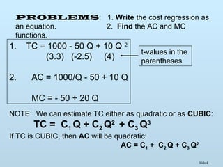
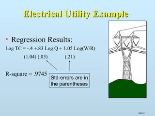
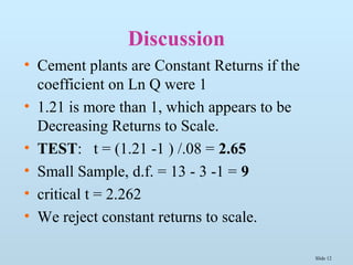
17. Slide 17
• Amount of sales
revenues that breaks
even
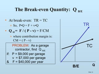
• P•QB/E = P•[F/(P-v)]
= F / [ 1 - v/P ]
Break-even Sales Volume
Variable Cost Ratio
Ex: At Q = 20,
B/E Sales Volume is
$9,000•20 =
$180,000 Sales Volume
Answer: Q = 40,000/(2,000)= 40/2 = 20
garages at the break-even point.

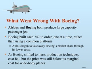
18. Slide 18
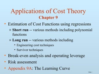
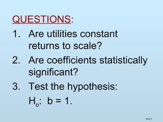
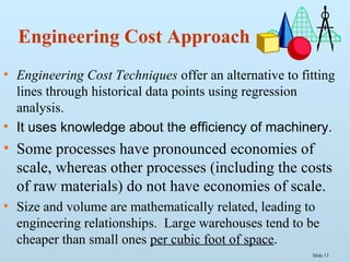
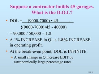
Target Profit Output
Quantity needed to attain a target
profit
If π is the target profit,
Q target π = [ F + π] / (P-v)
Suppose want to attain $50,000 profit, then,
Q target π = ($40,000 + $50,000)/$2,000
= $90,000/$2,000 = 45 garages

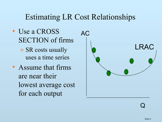
19. Slide 19
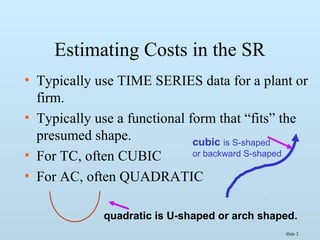
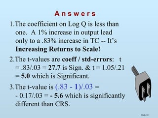
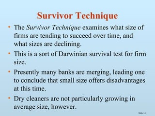
Degree of Operating Leverage
or Operating Profit Elasticity
• DOL = Eπ
» sensitivity of operating profit (EBIT) to
changes in output
• Operating π = TR-TC = (P-v)•Q - F
• Hence, DOL = ∂ π/∂ Q•(Q/π) =
(P-v)•(Q/π) = (P-v)•Q / [(P-v)•Q - F]
A measure of the importance of Fixed Cost
or Business Risk to fluctuations in output

20. Slide 20
Suppose a contractor builds 45 garages.
What is the D.O.L?
• DOL = (9000-7000) • 45 .
{(9000-7000)•45 - 40000}
= 90,000 / 50,000 = 1.8
• A 1% INCREASE in Q → 1.8% INCREASE
in operating profit.
• At the break-even point, DOL is INFINITE.
» A small change in Q increase EBIT by
astronomically large percentage rates

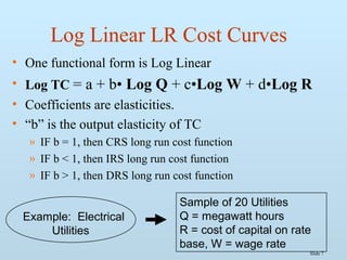
21. Slide 21
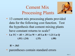
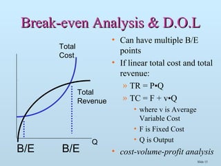
DOL as
Operating Profit Elasticity
DOL = [ (P - v)Q ] / { [ (P - v)Q ] - F }
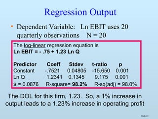
• We can use empirical estimation methods to find
operating leverage
• Elasticities can be estimated with double log
functional forms
• Use a time series of data on operating profit and
output
» Ln EBIT = a + b• Ln Q, where b is the DOL
» then a 1% increase in output increases EBIT by b%
» b tends to be greater than or equal to 1

22. Slide 22
Regression Output
• Dependent Variable: Ln EBIT uses 20
quarterly observations N = 20
The log-linear regression equation is
Ln EBIT = - .75 + 1.23 Ln Q
Predictor Coeff Stdev t-ratio p
Constant -.7521 0.04805 -15.650 0.001
Ln Q 1.2341 0.1345 9.175 0.001
s = 0.0876 R-square= 98.2% R-sq(adj) = 98.0%
The DOL for this firm, 1.23. So, a 1% increase in
output leads to a 1.23% increase in operating profit

23. Slide 23
Operating Profit and the Business Cycle
Output
recession
TIME
EBIT =
operating
profit
Trough
peak
1. EBIT is more volatile
that output over cycle
2. EBIT tends to
collapse late in
recessions

24. Slide 24
Learning Curve: Appendix 9A
• “Learning by doing” has wide application in
production processes.
• Workers and management become more efficient with
experience.
• the cost of production declines as the
accumulated past production, Q = Σqt,
increases, where qt is the amount produced in
the tth
period.
• Airline manufacturing, ship building, and appliance
manufacturing have demonstrated the learning curve
effect.

25. Slide 25
• Functionally, the learning curve relationship can
be written C = a·Qb
, where C is the input cost of
the Qth unit:
• Taking the (natural) logarithm of both sides, we
get: log C = log a + b·log Q
• The coefficient b tells us the extent of the
learning curve effect.
» If the b=0, then costs are at a constant level.
» If b > 0, then costs rise in output, which is exactly
opposite of the learning curve effect.
» If b < 0, then costs decline in output, as predicted by
the learning curve effect.