Downloaded 402 times
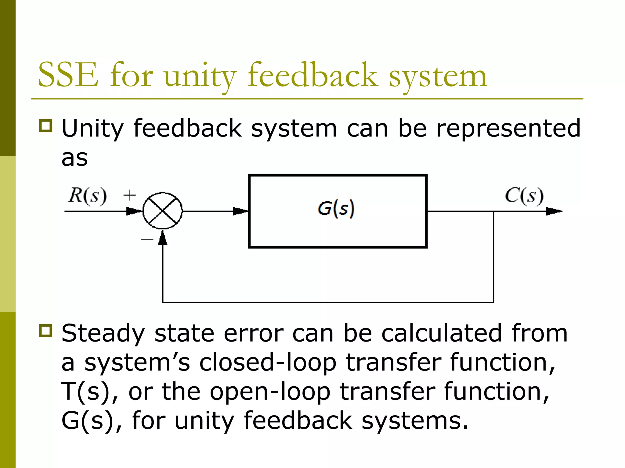
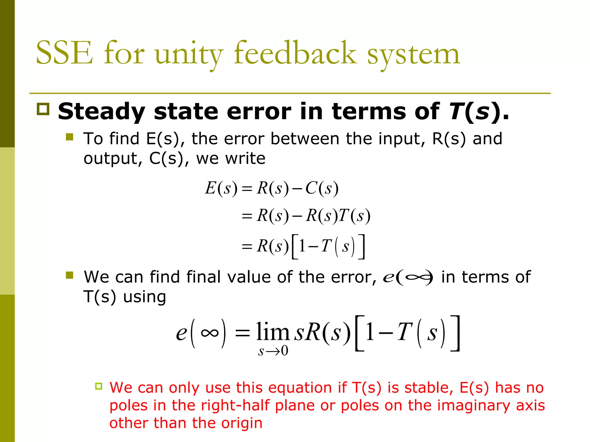

This document discusses steady-state errors in control systems. It defines steady-state error as the difference between the input and output of a system as time approaches infinity. For a unity feedback system, the steady-state error can be calculated from the closed-loop transfer function T(s) or open-loop transfer function G(s). The steady-state error depends on the type of input signal (step, ramp, or parabola) and number of integrations in the system. Systems are classified as Type 0, 1, or 2 based on this number of integrations. The document provides examples of calculating steady-state error for different system types and input signals.
Overview of control systems theory focusing on forced response errors including objectives for analyzing steady-state error.
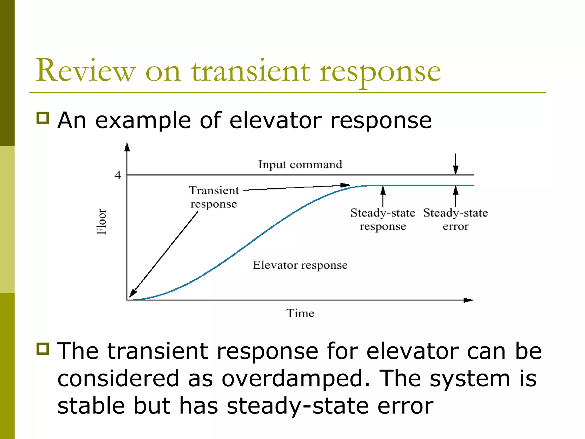
Recap on types of transient response in second-order systems with an example relating to elevators.
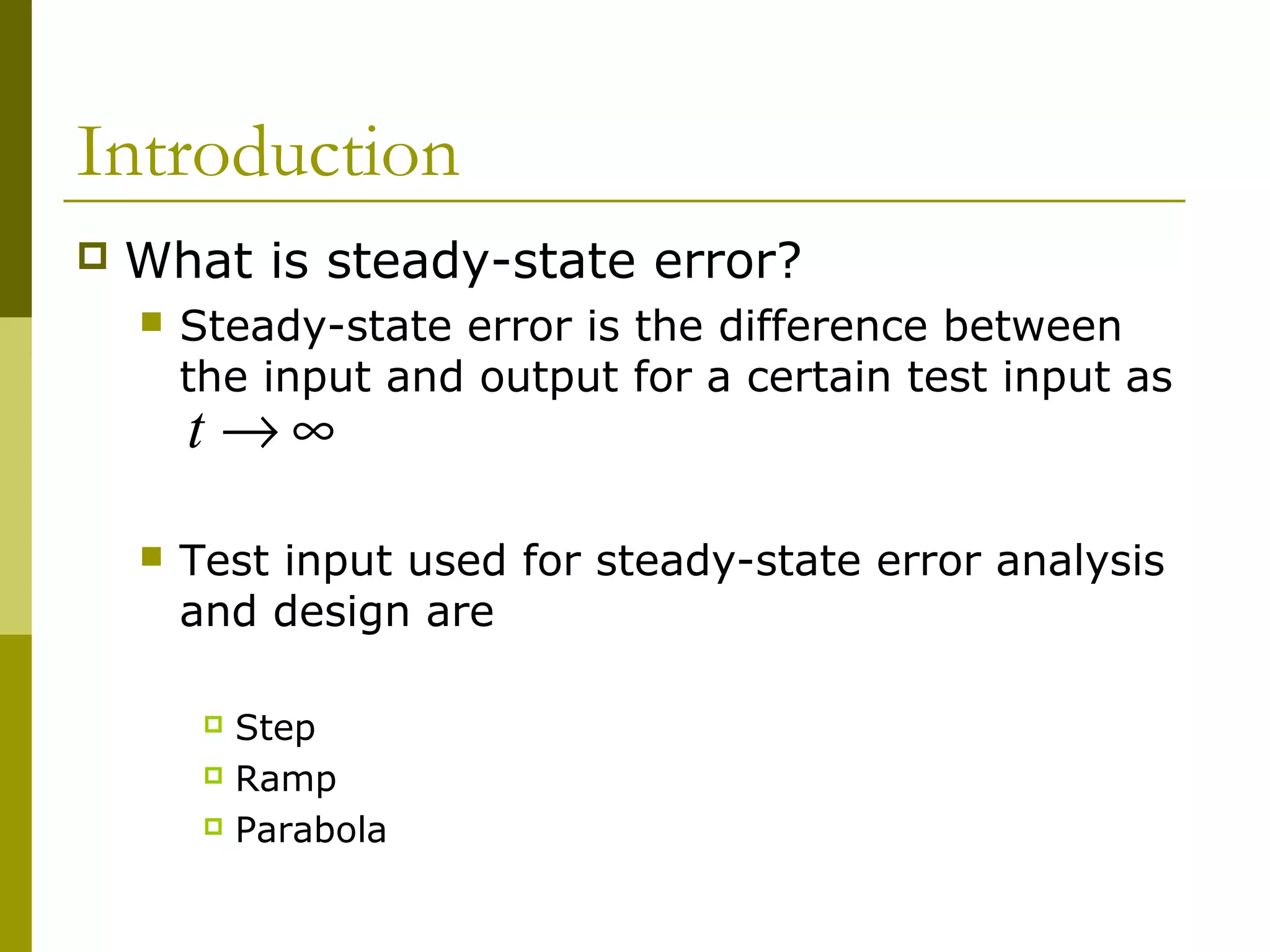
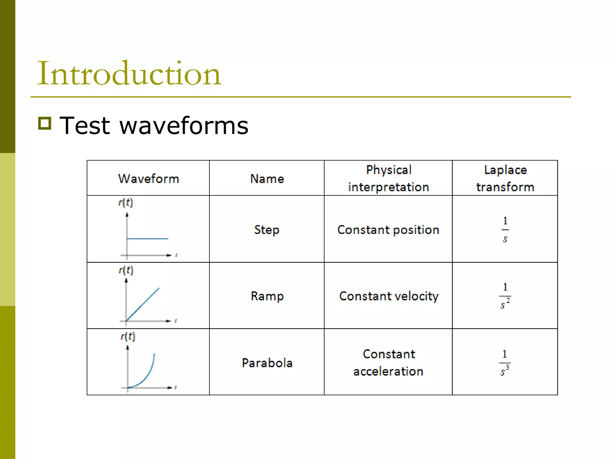
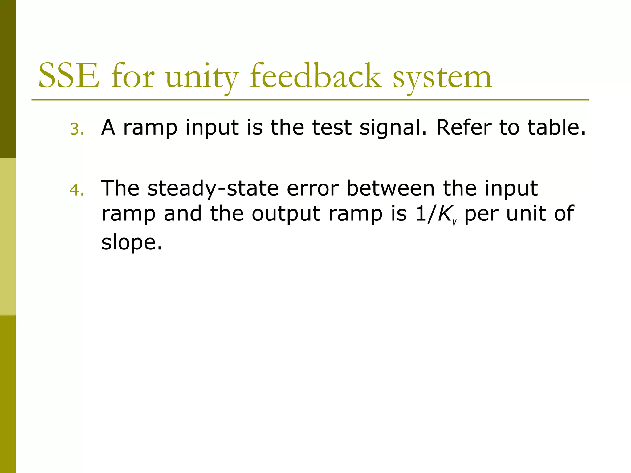
Explanation of steady-state error (SSE) and testing methods involving step, ramp, and parabola inputs.
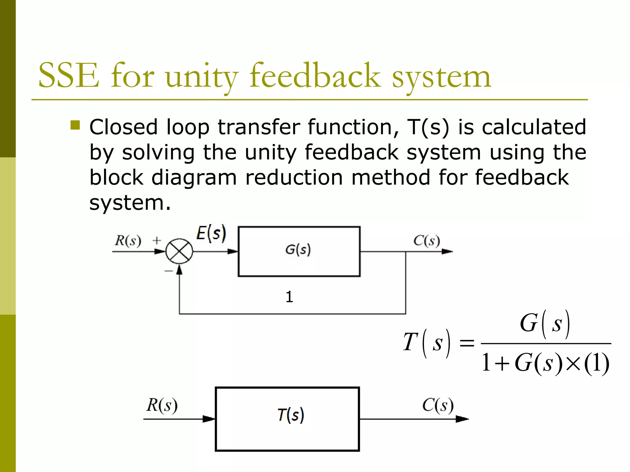
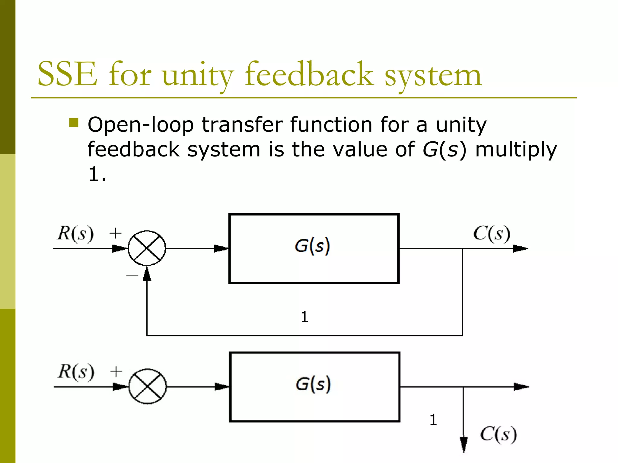
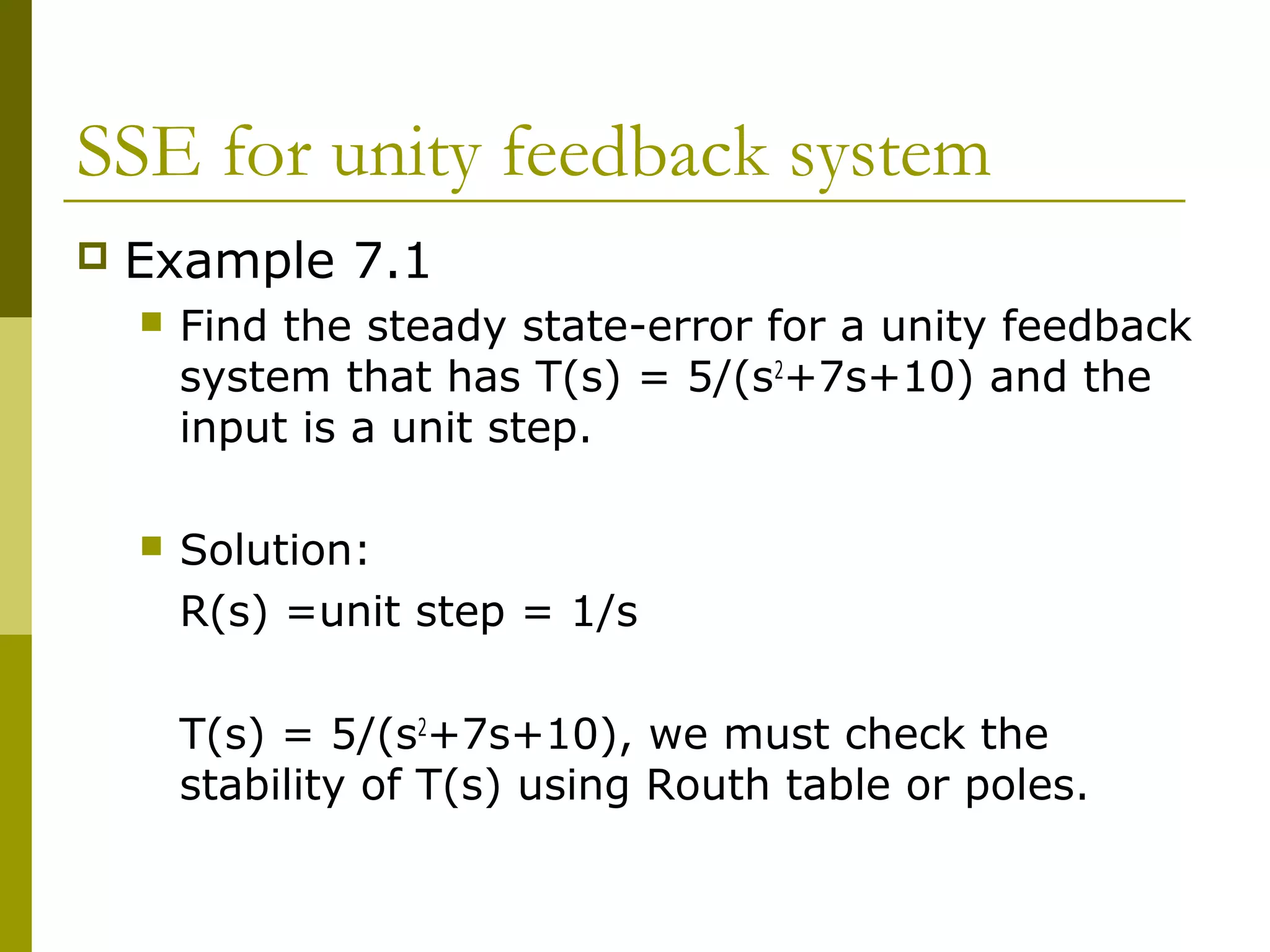
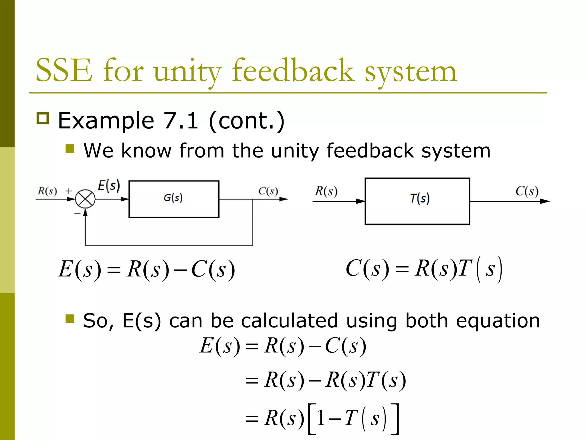
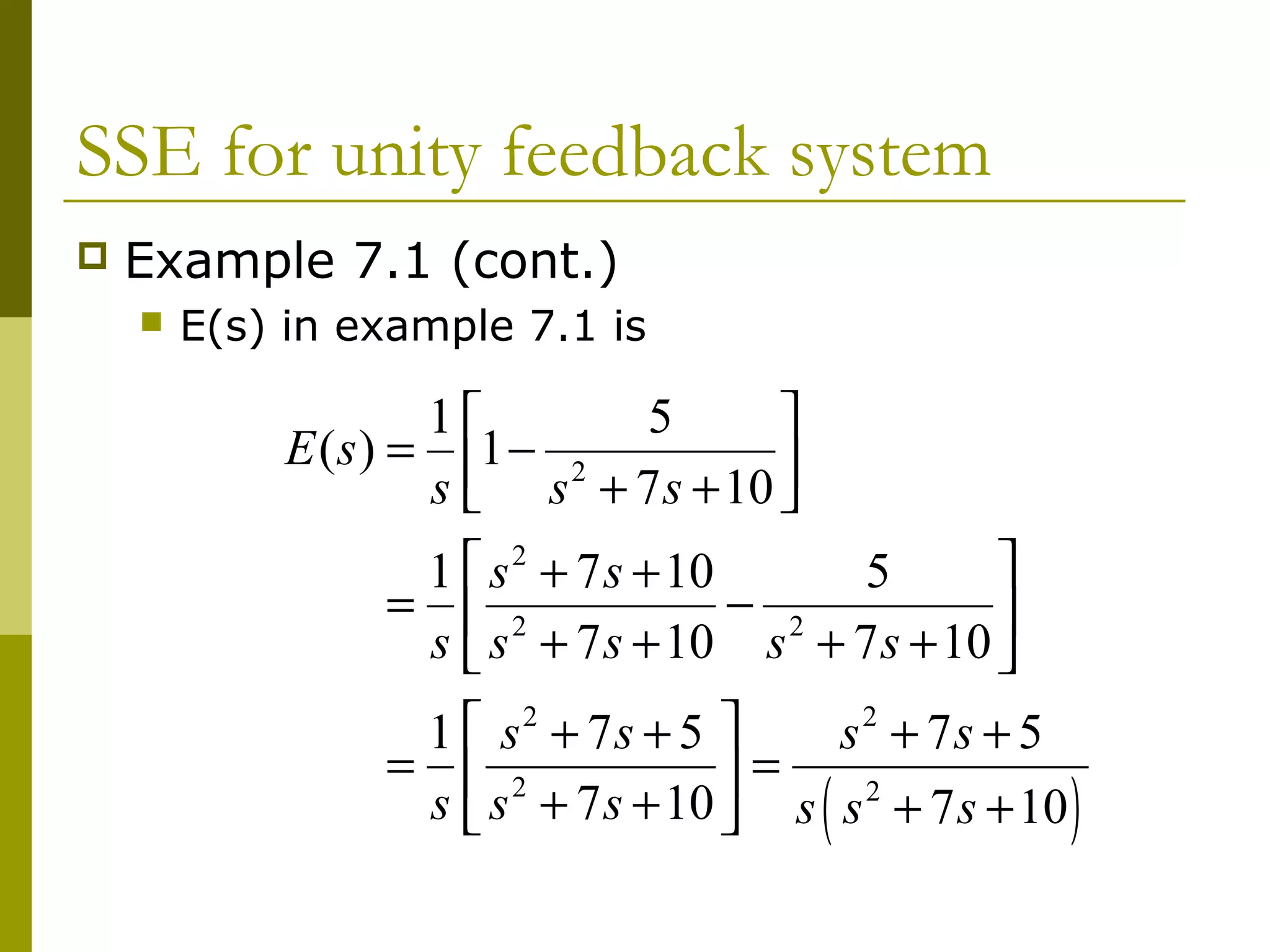
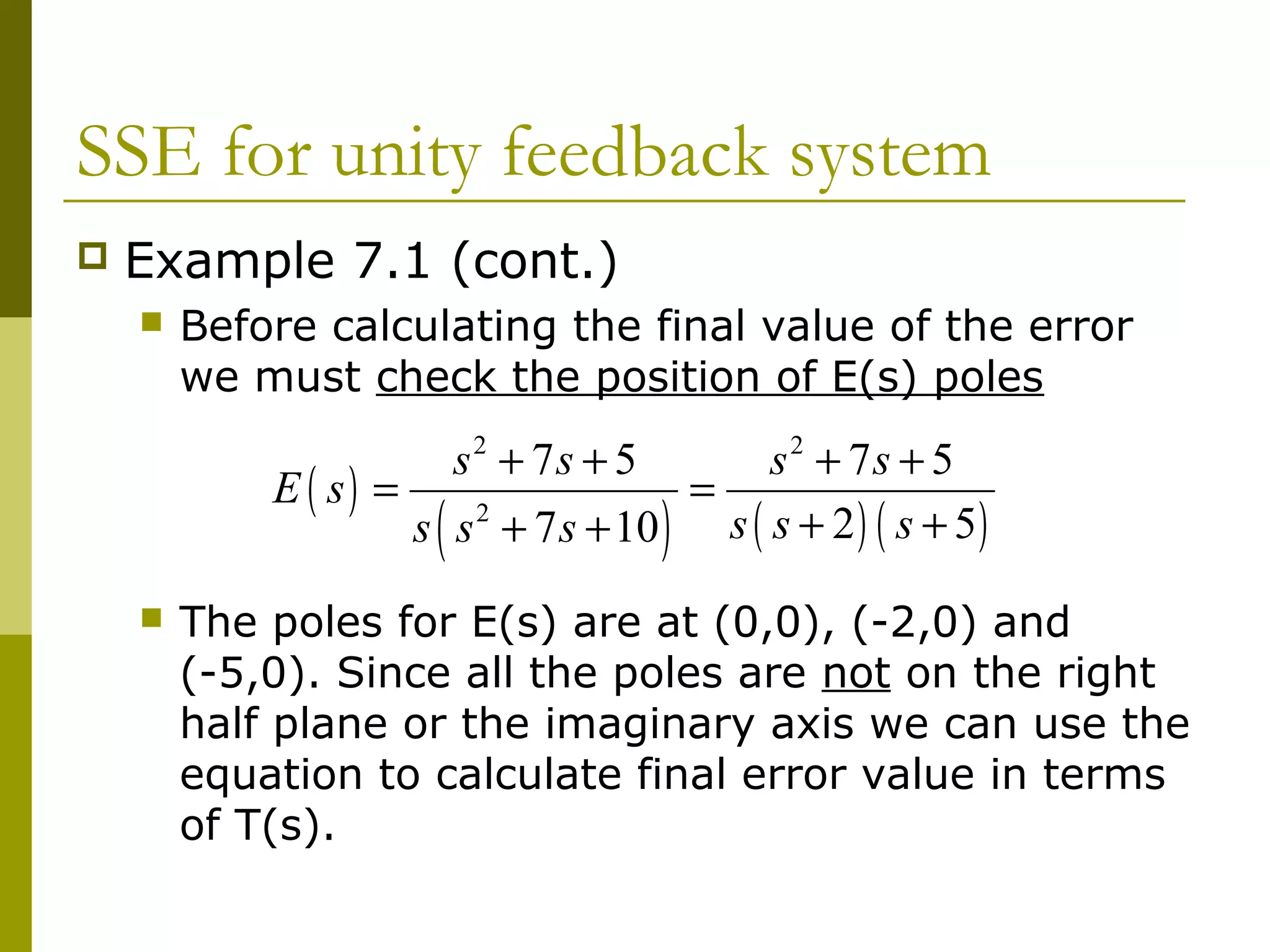
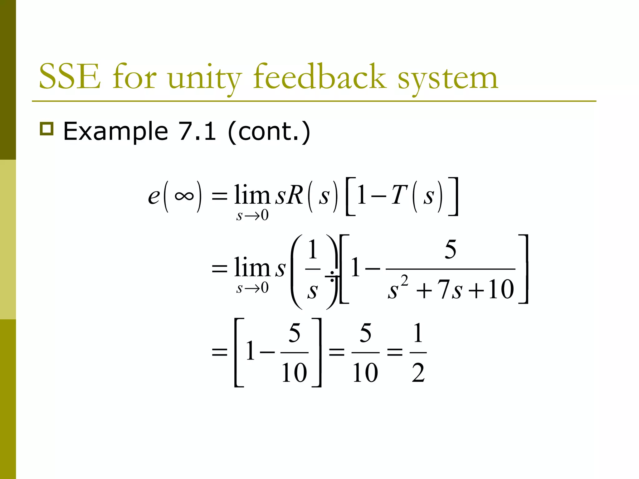
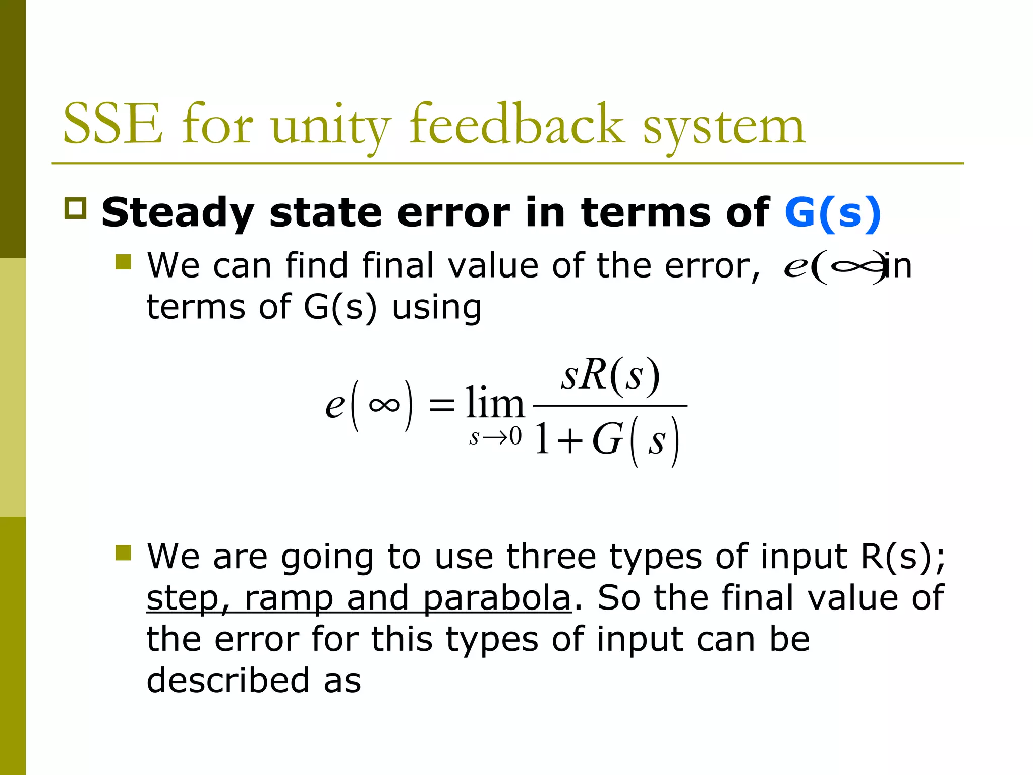
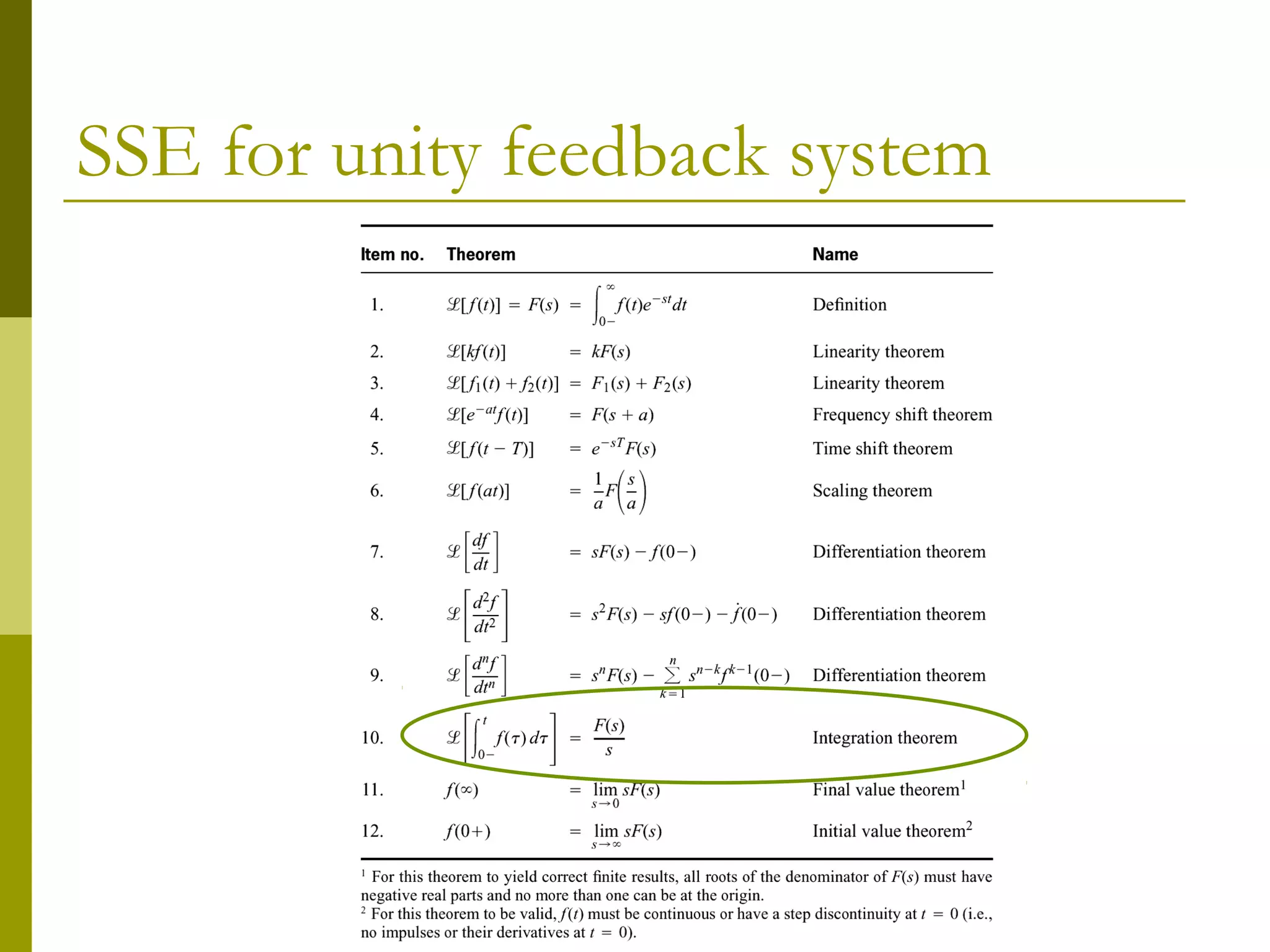
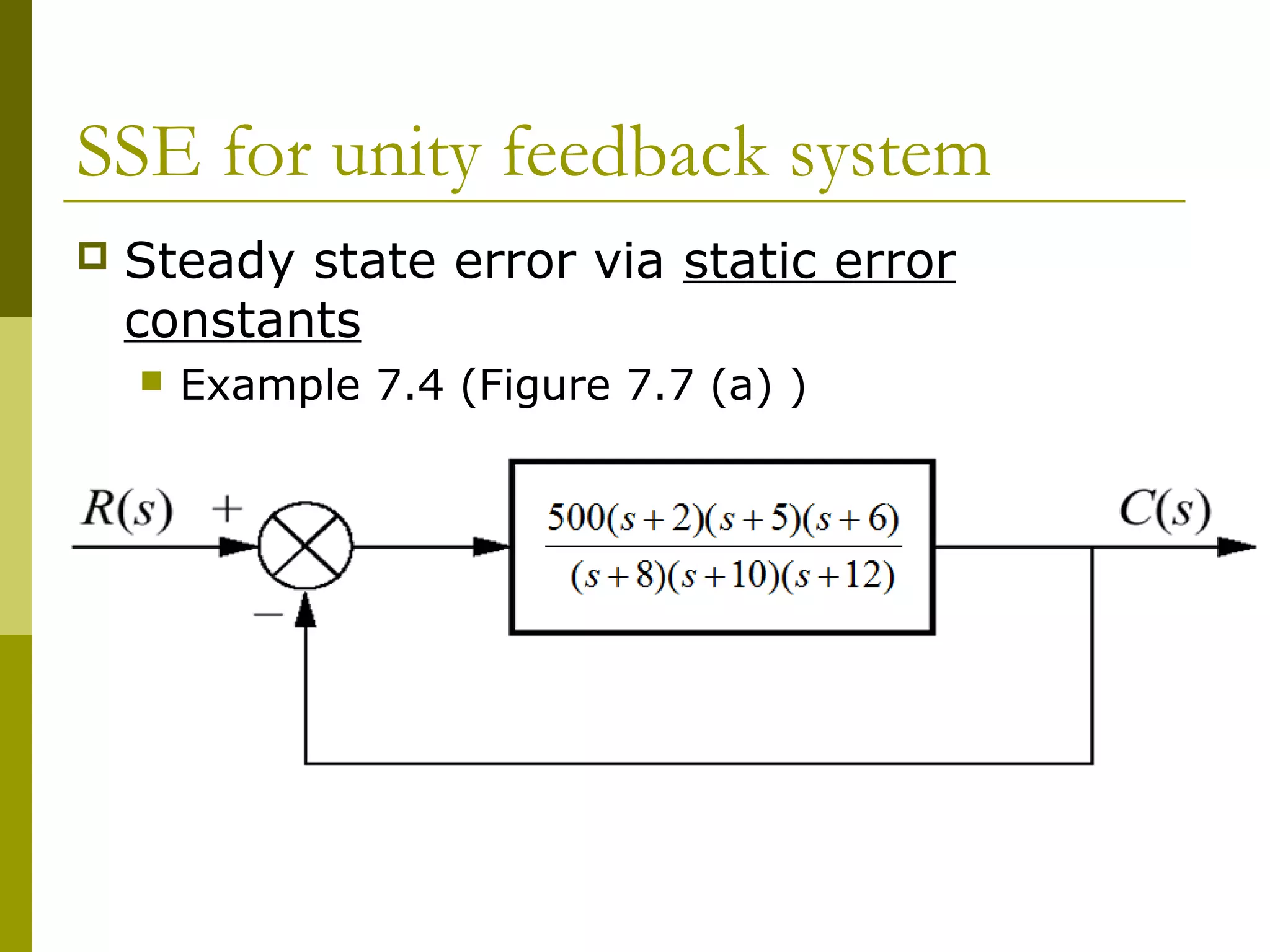
Calculation of SSE for unity feedback using closed-loop and open-loop transfer functions.
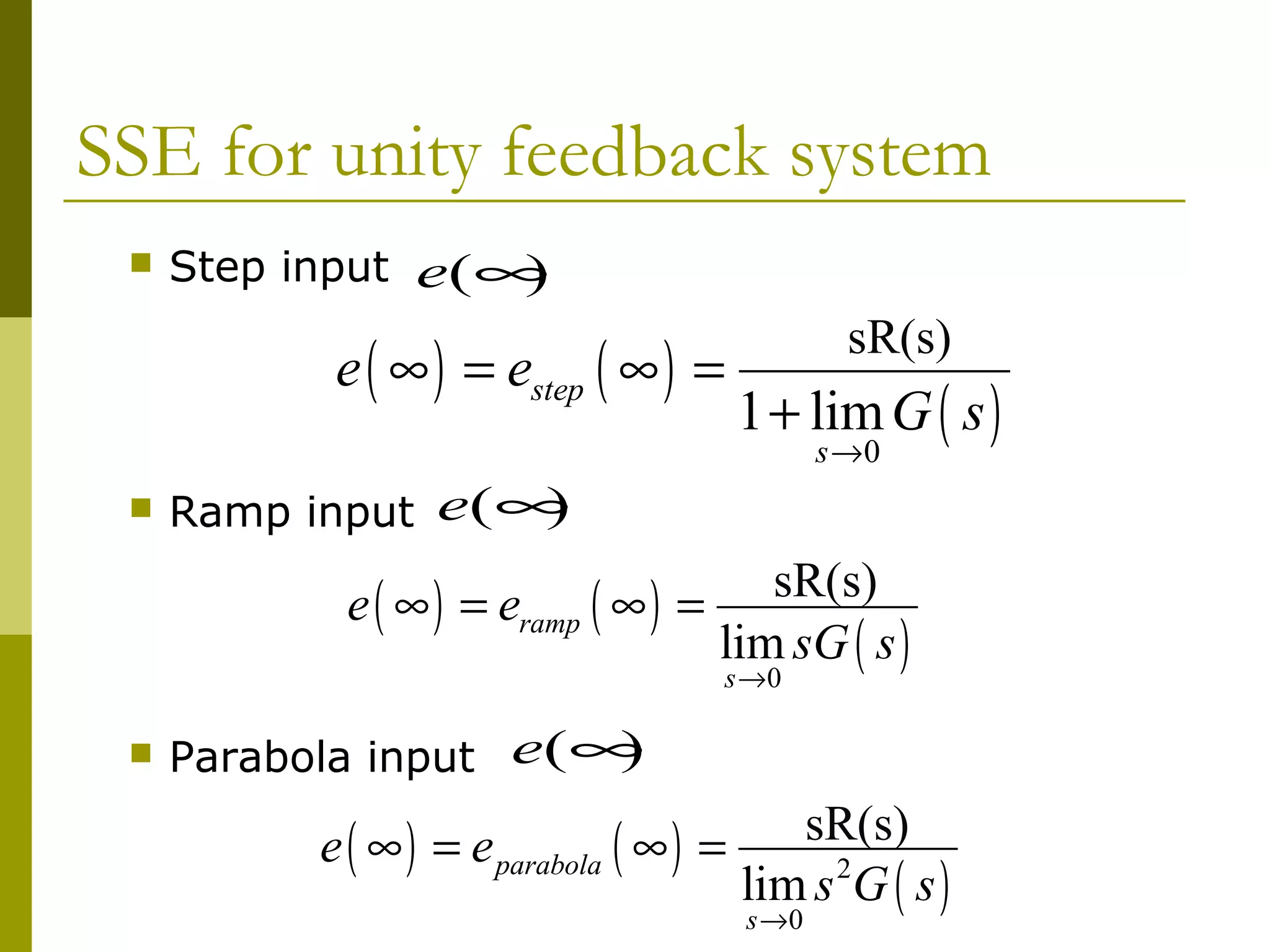
Derivation and calculation methods for SSE using formulas and examples, focusing on system stability.
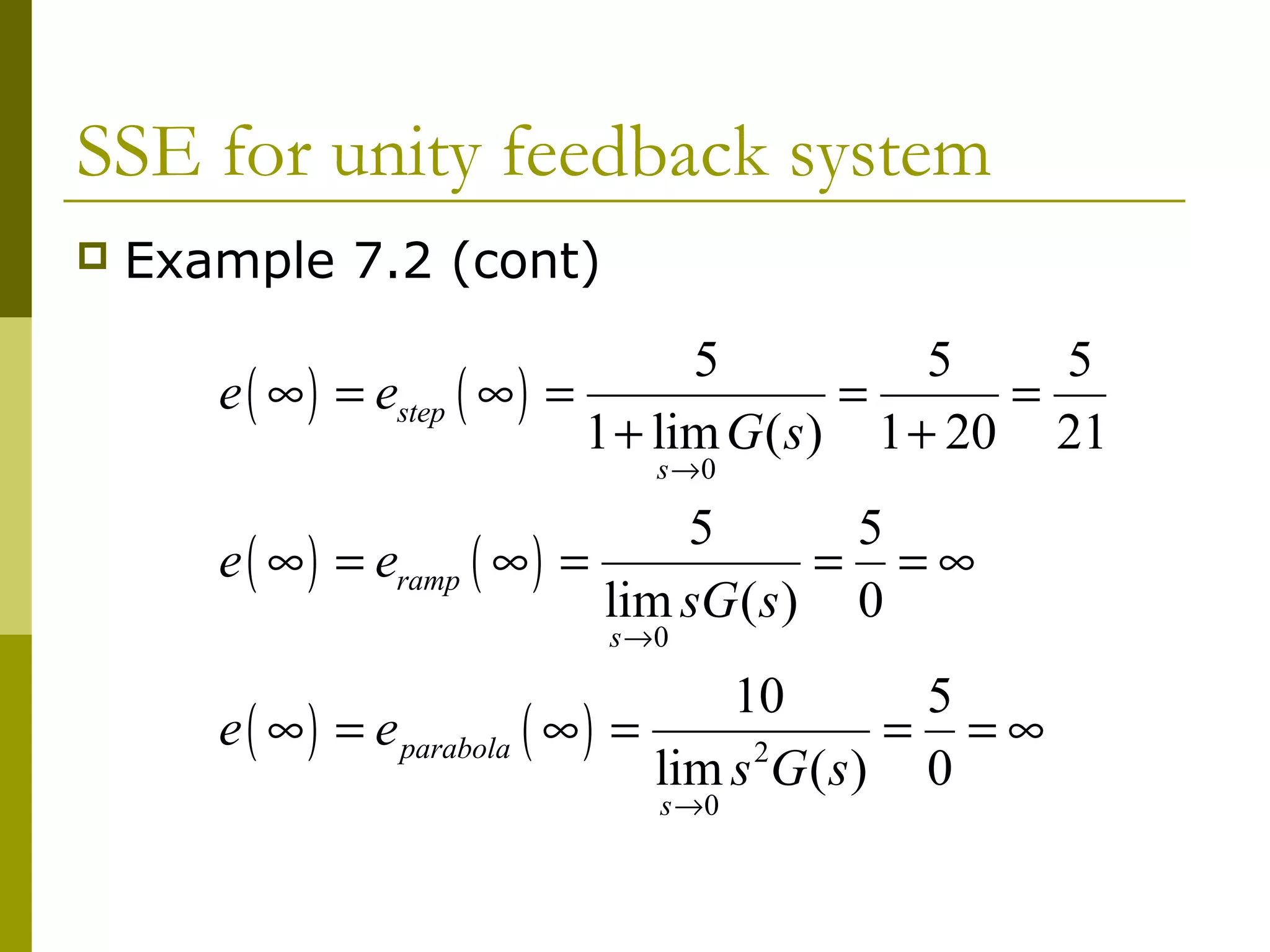
Exemplification of SSE calculations for step, ramp, and parabola inputs, highlighting results across inputs.
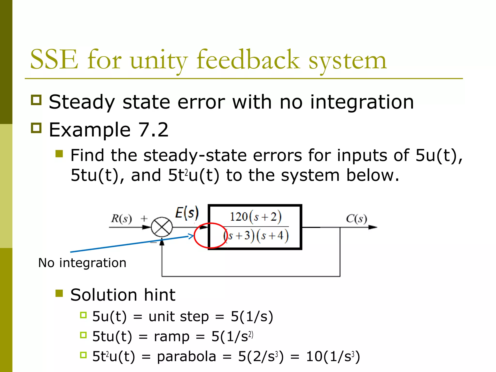
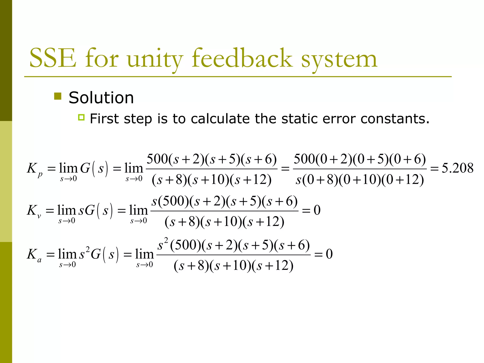
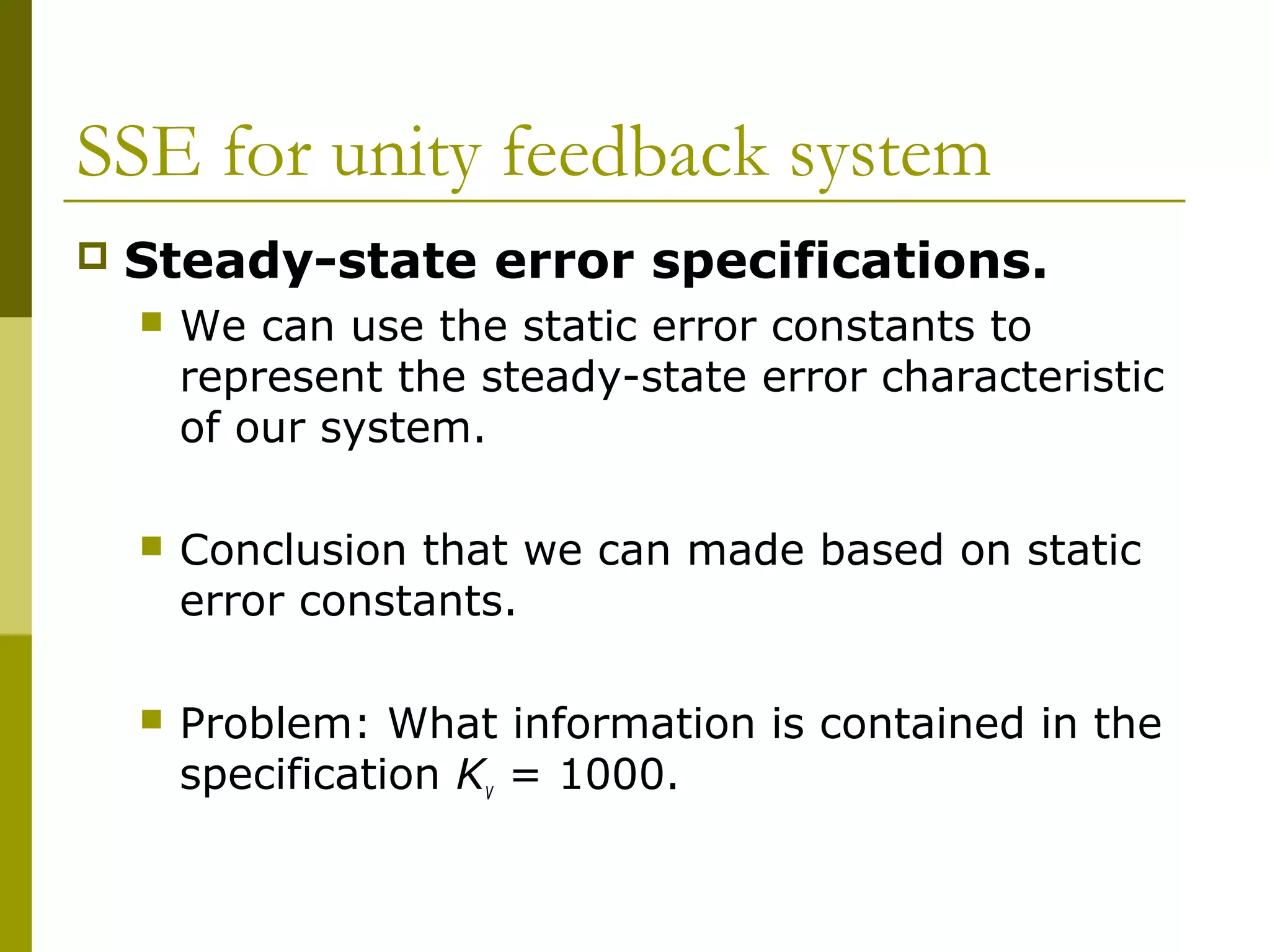
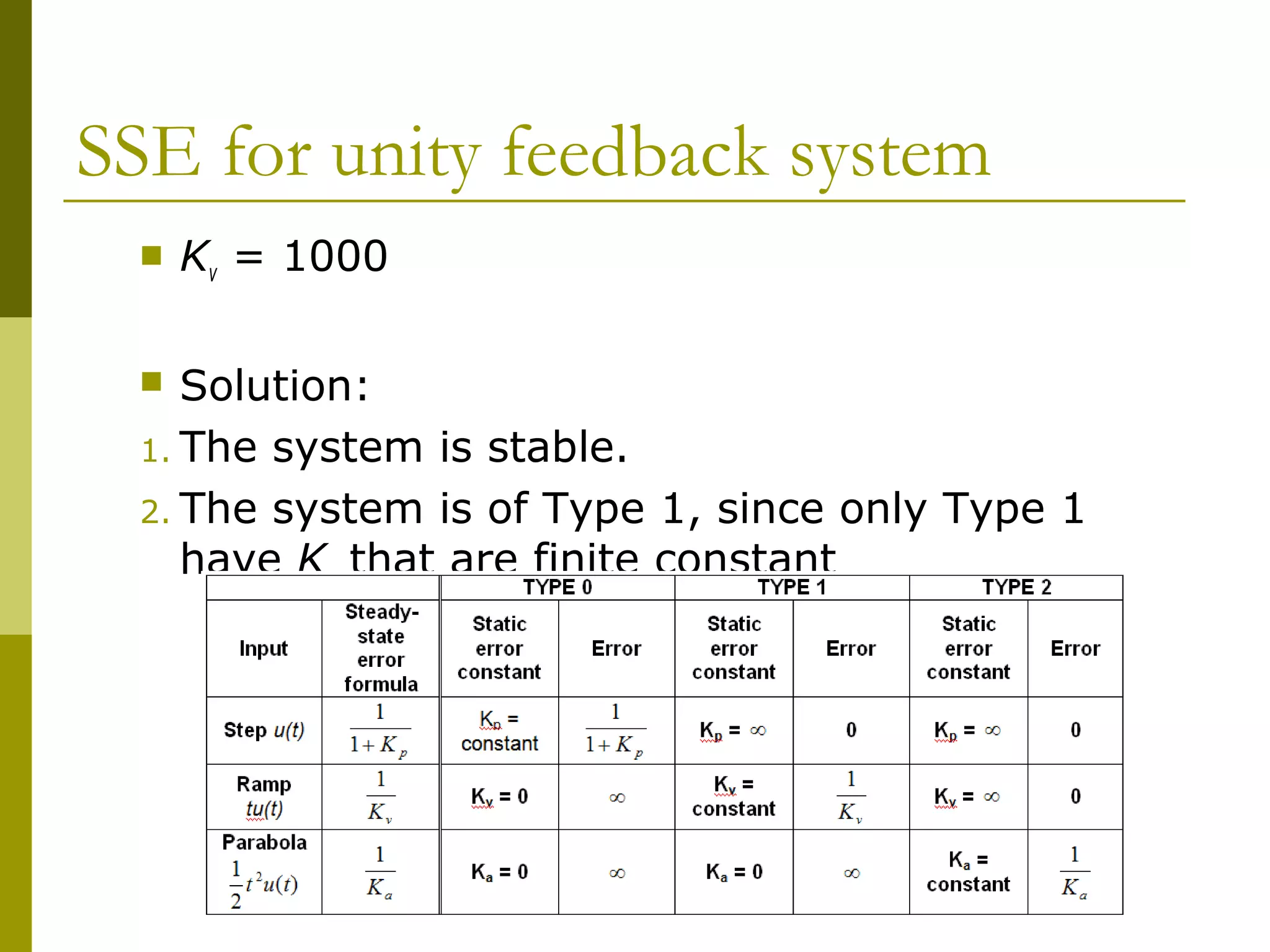
Further challenges on SSEs and highlights concepts surrounding static error constants.
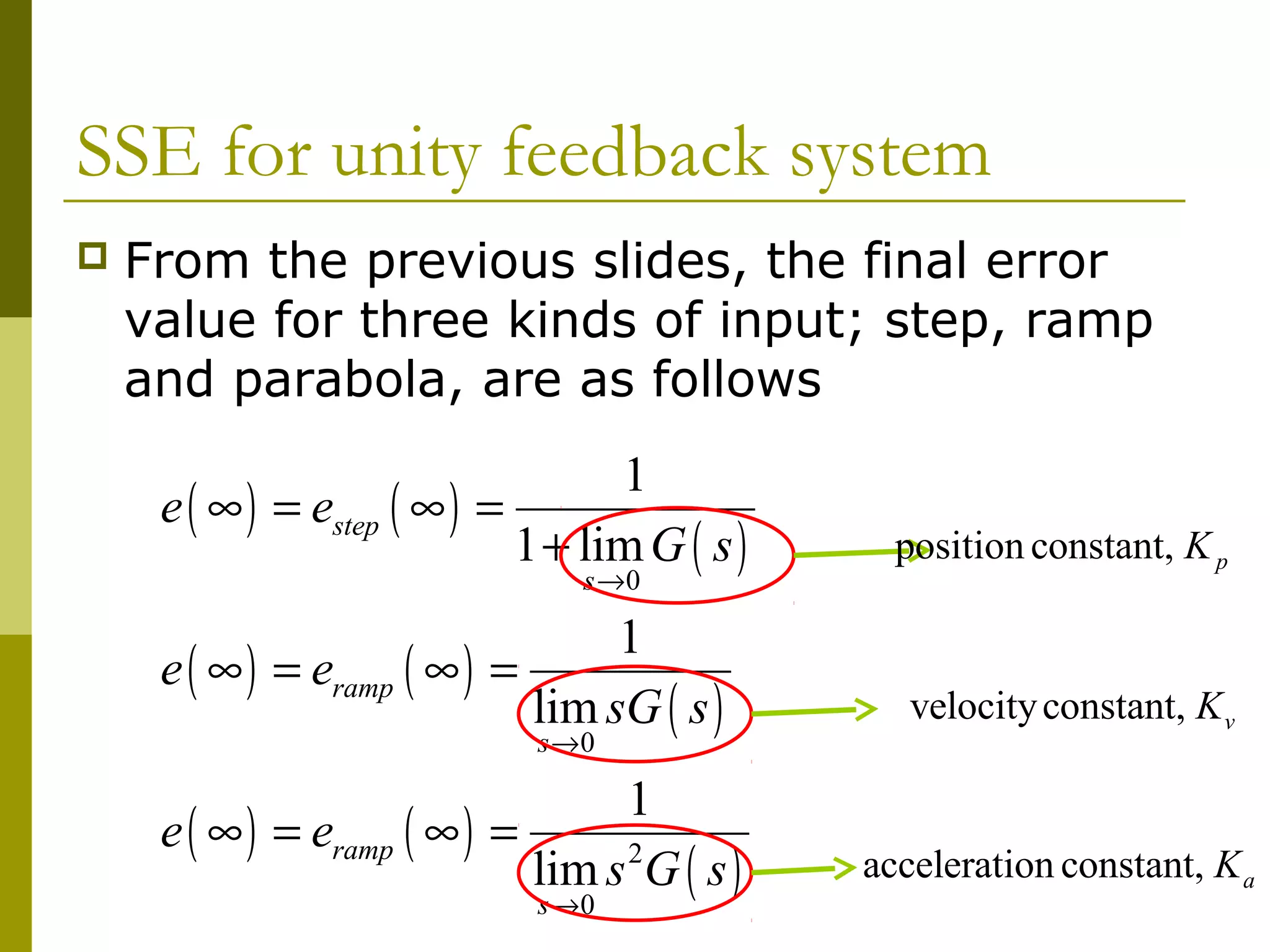
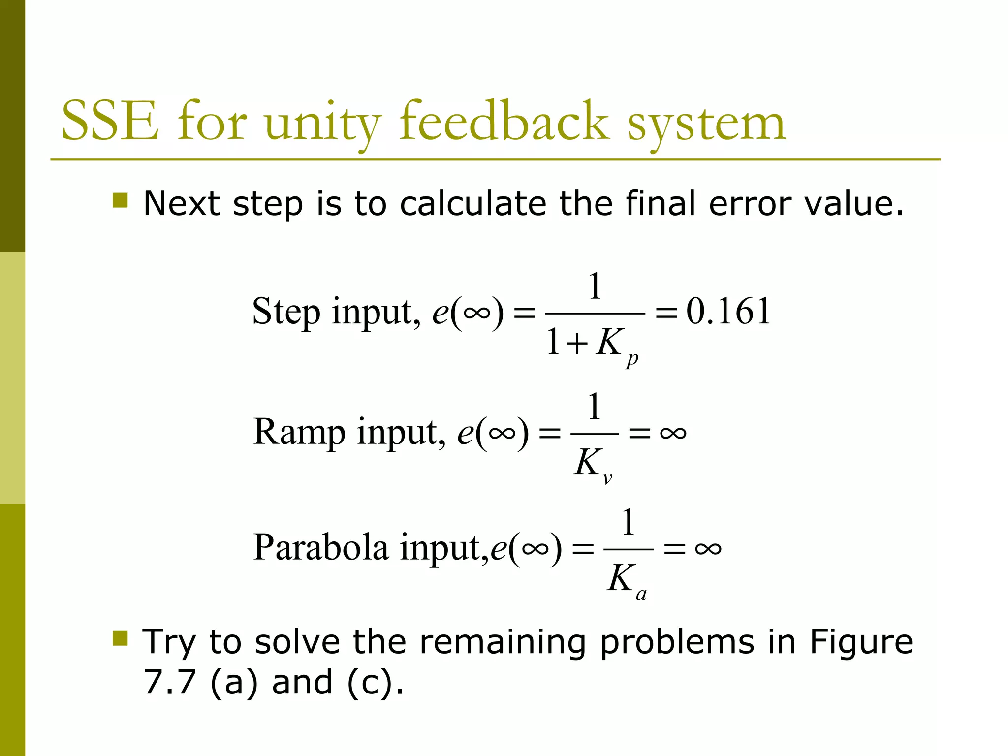
Determining final error values through static error constants for distinct input types in systems.
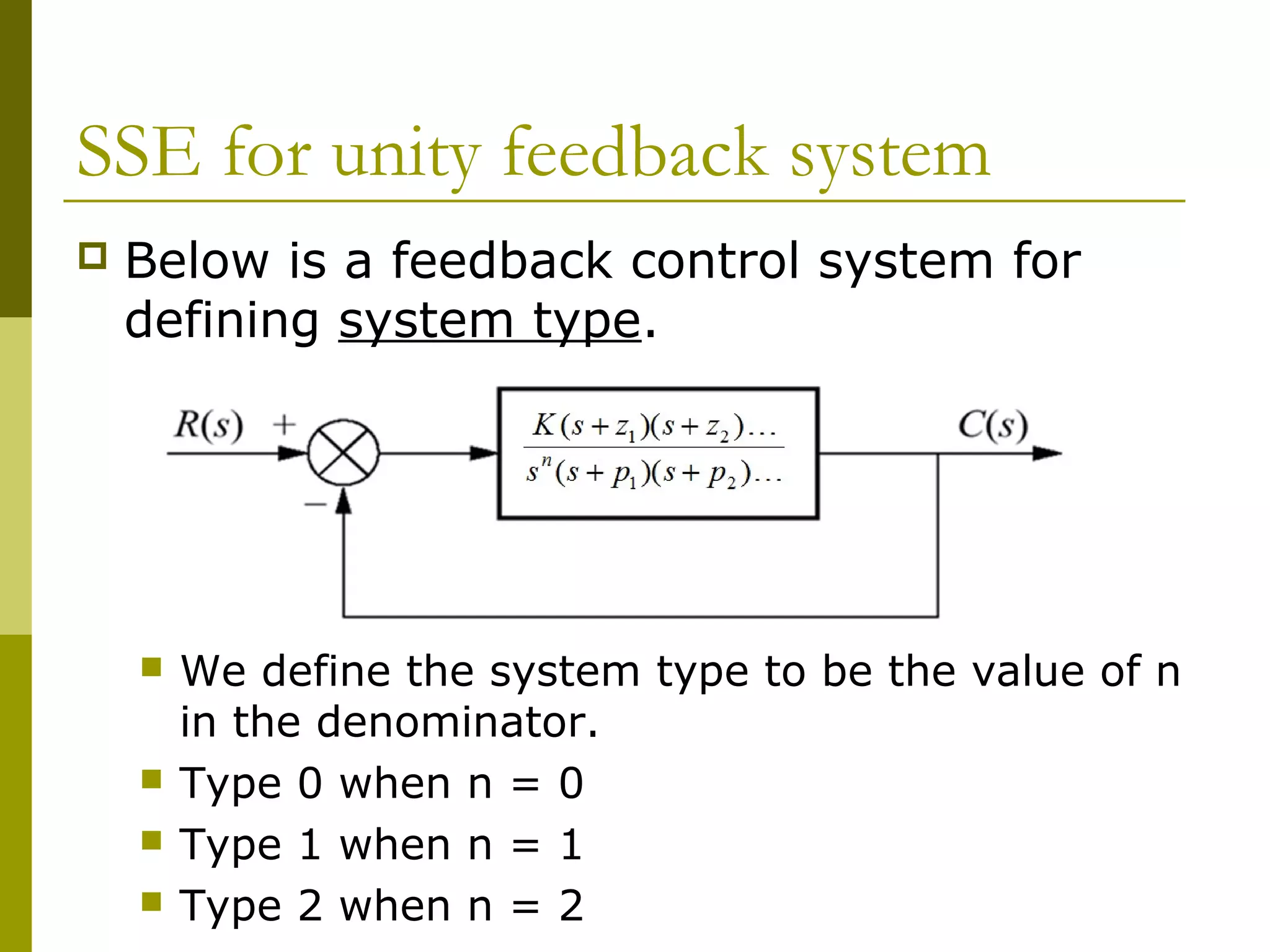
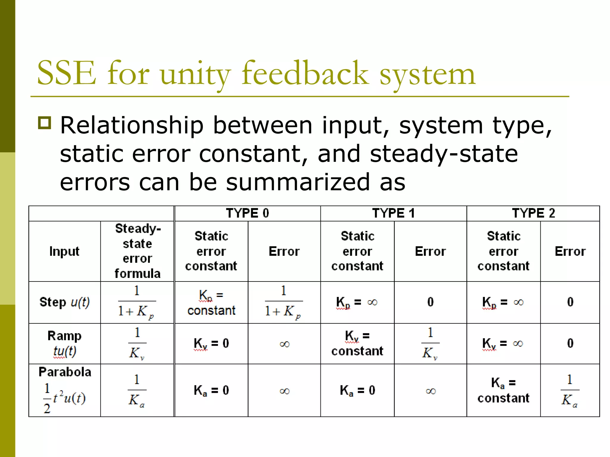
Defining system types based on integrations affecting SSE, and illustrating specifications and conclusions from static error constants.