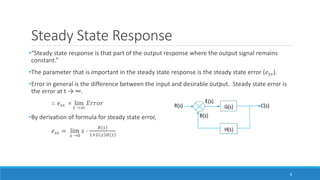
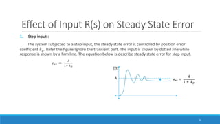
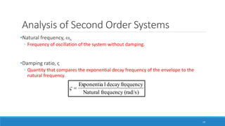
The document discusses time response analysis in control systems, focusing on how different input types (impulse, step, ramp, parabolic, and sinusoidal) affect output responses. It explains the concept of steady state response and steady state error, detailing how these are influenced by the type of system and the input applied. Additionally, the document covers transient response and specifications such as delay time, rise time, peak time, and overshoot.

1. Time Response Analysis
BY KAUSHAL PATEL

2. What is Time Response?
•Time response of system is defined as the output of a system when subjected when to an input
which is a functions of time.
•In the block diagram representation and signal flow graphs we studied how to obtain the
transfer function of a physical system. We have also seen how to combine individual transfer
functions to get a single transfer function using block diagram reduction and signal flow graphs.
We shall now study how this block responds to different inputs, i.e. we will now take closer look
at the response characteristics of the control system.
2

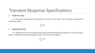
3. Inputs Supplied to a System
1. Impulse input :
Impulse represents a sudden change in input. An Impulse is infinite at t = 0 and zero
everywhere else. The area under the curve is 1. A unit impulse has magnitude 1 at t = 0.
r(t) = δ(t) = 1 t = 0
= 0 t ≠ 0
In the Laplace domain we have
L[r(t)] = L[δ(t)] = 1
Impulse inputs are used to derived a mathematical model of the system.
3

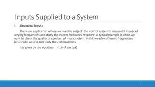
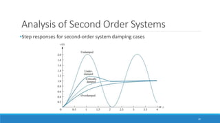
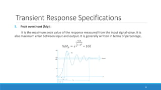
4. Inputs Supplied to a System
2. Step input :
A step input represents a constant command such as position. The input given to an elevator
is step input. Another example of a step input is setting the temperature of an air
conditioner.
A step signal is given by the formula,
r(t) = u(t) = A t ≥ 0
= 0 otherwise , If A = 1, it is called step.
In Laplace domain, we have
L[r(t)] = R(s) =
𝐴
𝑠
In case of a unit step, we get L [ r(t)] = R(s) =
1
𝑠
4

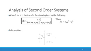
5. Inputs Supplied to a System
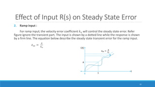
3. Ramp input :
The ramp input represents a linearly increasing input command. It is given by the formula,
r(t) = At t ≥ 0 ; Here A is the slope.
= 0 t < 0
If A = 1, it is called a unit ramp.
In the Laplace domain we have,
L [r(t)] = R(s) =
𝐴
𝑠2
In case of unit ramp, we have R(s) =
1
𝑠2
System are subjected to Ramp inputs when we need to study the system behavior for linear
increasing functions like velocity.
5

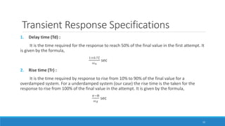
6. Inputs Supplied to a System
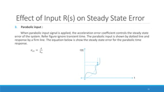
4. Parabolic input :
Rate of change of velocity is acceleration. Acceleration is a parabolic function. It is given by
the formula,
r(t) =
𝐴𝑡2
2
t ≥ 0
= 0 t < 0
If A = 1, it is called a unit parabola. In the Laplace domain we have
L [r(t)] = R(s) =
𝐴
𝑠3
In case of unit parabola, we have R(s) =
1
𝑠3
6

7. Inputs Supplied to a System
5. Sinusoidal input :
There are application where we need to subject the control system to sinusoidal inputs of
varying frequencies and study the system frequency response. A typical example is when we
want to check the quality of speakers of music system. In this we play different frequencies
(sinusoidal waves) and study their attenuations.
It is given by the equation, r(t) = A sin (ωt)
7

8. Steady State Response
•“Steady state response is that part of the output response where the output signal remains
constant.”
•The parameter that is important in the steady state response is the steady state error (𝑒𝑠𝑠).
•Error in general is the difference between the input and desirable output. Steady state error is
the error at t → ∞.
∴ 𝑒𝑠𝑠 = lim
𝑡 →∞
𝐸𝑟𝑟𝑜𝑟
•By derivation of formula for steady state error,
𝑒𝑠𝑠 = lim
𝑠 →0
𝑠 ∙
𝑅(𝑠)
1+𝐺 𝑠 𝐻(𝑠)
8

9. Effect of Input R(s) on Steady State Error
1. Step input :
The system subjected to a step input, the steady state error is controlled by position error
coefficient 𝑘 𝑝. Refer the figure Ignore the transient part. The input is shown by dotted line while
response is shown by a firm line. The equation below is describe steady state error for step input.
𝑒𝑠𝑠 =
𝐴
1+ 𝑘 𝑝
9

10. Effect of Input R(s) on Steady State Error
2. Ramp input :
For ramp input; the velocity error coefficient 𝑘 𝑣 will control the steady state error. Refer
figure ignore the transient part. The input is shown by a dotted line while the response is shown
by a firm line. The equation below describe the steady state transient error for the ramp input.
𝑒𝑠𝑠 =
𝐴
𝑘 𝑣
10

11. Effect of Input R(s) on Steady State Error
3. Parabolic input :
When parabolic input signal is applied, the acceleration error coefficient controls the steady state
error of the system. Refer figure ignore transient time. The parabolic input is shown by dotted line and
response by a firm line. The equation below is show the steady state error for the parabolic time
response.
𝑒𝑠𝑠 =
𝐴
𝑘 𝑎
11

12. Effect of Open Loop Transfer Function on
Steady State Error
•The steady state error(𝑒𝑠𝑠) also depends on G(s)H(s). Actually 𝑒𝑠𝑠 depends on the Type of system
G(s)H(s).
•Type of system is defined by the number of open loop Poles i.e., poles of G(s)H(s) that are present at
the origin.
•The open loop transfer function written in time constant form is,
𝐺 𝑠 𝐻 𝑠 =
𝑘1 1+𝑇𝑧1 𝑠 1+𝑇𝑧2 𝑠 …
𝑠 𝑛 1+𝑇𝑝1 𝑠 1+𝑇𝑝2 𝑠 …
•The open loop transfer function written in pole-zero form is written as
𝐺 𝑠 𝐻 𝑠 =
𝑘 𝑠+𝑧1 𝑠+𝑧2 …
𝑠 𝑛 𝑠+𝑝1 𝑠+𝑝2 …
•Here n is number of poles at the origin. It is very easy to obtain one from the other.
12

13. Subjecting a Type 0,1 & 2 Systems to a
Step, Ramp & Parabolic Input
Sr. No. Type Step Input Ramp Input Parabolic Input
𝒌 𝒑 𝒆 𝒔𝒔 𝒌 𝒗 𝒆 𝒔𝒔 𝒌 𝒂 𝒆 𝒔𝒔
(1) Type Zero K 𝐴
1 + 𝑘
0 ∞ 0 ∞
(2) Type One ∞ 0 k 𝐴
𝑘
0 ∞
(3) Type Two ∞ 0 ∞ 0 K 𝐴
𝑘
13

14. Transient Response
•In the earlier section, we discussed the steady state response in detail and found a method of
calculating the steady state error.
•We realized that 𝑒𝑠𝑠 was dependent on the Type of the system i.e. the number of poles, the
system had at the origin.
•The transient response of the system depends on the order of system. Order of a system is the
highest power of s in the denominator of closed loop transfer function.
•Hence for transient response, we need to work with the closed loop transfer function,
𝐺(𝑠)
1+𝐺 𝑠 𝐻(𝑠)
14

15. Analysis of First Order Systems
15
•General form:
•Problem: Derive the transfer function for the following circuit
1)(
)(
)(


s
K
sR
sC
sG

1
1
)(


RCs
sG

16. 16
Analysis of First Order Systems
•Transient Response: Gradual change of output from initial to the desired
condition.
•Block diagram representation:
•By definition itself, the input to the system should be a step function which is
given by the following:
C(s)R(s)
1s
K

s
sR
1
)( 
Where,
K : Gain
 : Time constant

17. 17
Analysis of First Order Systems
•General form:
•Output response:
1)(
)(
)(


s
K
sR
sC
sG

1
1
1
)(
















s
B
s
A
s
K
s
sC




t
e
B
Atc 
)(
)()()( sRsGsC 

18. Analysis of Second Order Systems
18
•General form:
•Roots of denominator:
  22
2
2 nn
n
ss
K
sG




Where,
K : Gain
ς : Damping ratio
n : Undamped natural frequency
02 22
 nnss 
12
2,1   nns

19. 19
Analysis of Second Order Systems
•Natural frequency, n
◦ Frequency of oscillation of the system without damping.
•Damping ratio, ς
◦ Quantity that compares the exponential decay frequency of the envelope to the
natural frequency.
(rad/s)frequencyNatural
frequencydecaylExponentia


20. Analysis of Second Order Systems
20
•Step responses for second-order system damping cases

21. Analysis of Second Order Systems
21
•When 0 < ς < 1, the transfer function is given by the following.
•Pole position:
 
  dndn
n
jsjs
K
sG




2 Where,
2
1   nd

22. Transient Response Specifications
1. Delay time (Td) :
It is the time required for the response to reach 50% of the final value in the first attempt. It
is given by the formula,
1+0.7𝜉
𝜔 𝑛
sec
2. Rise time (Tr) :
It is the time required by response to rise from 10% to 90% of the final value for a
overdamped system. For a underdamped system (our case) the rise time is the taken for the
response to rise from 100% of the final value in the attempt. It is given by the formula,
𝜋−Θ
𝜔 𝑑
sec
22

23. Transient Response Specifications
3. Peak time (Tp) :
It is the time required by the response to reach its first peak. The first peak is always the
maximum peak,
𝜋
𝜔 𝑑
sec
4. Setting time (Ts) :
It is defined as the time required for the transient damped oscillations to reach and stay
within a specified tolerance band (usually 2% of the input value).
4
𝜉𝜔 𝑛
sec
23

24. Transient Response Specifications
5. Peak overshoot (Mp) :
It is the maximum peak value of the response measured from the input signal value. It is
also maximum error between input and output. It is generally written in terms of percentage,
%𝑀 𝑝 = 𝑒
−𝜉𝜋
1−𝜉2
∗ 100
24

25. Thank You