Time-Response Lecture

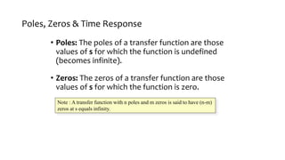
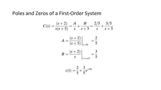
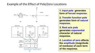
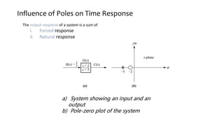
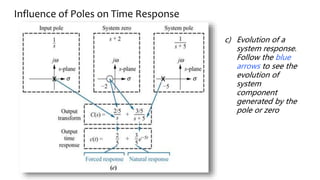
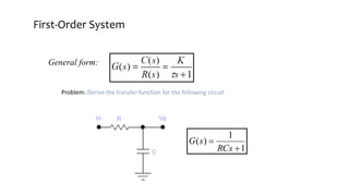
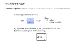
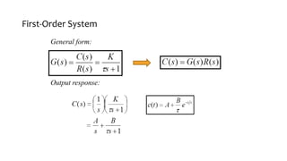
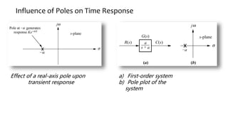
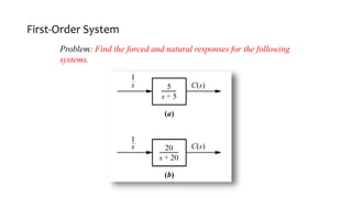
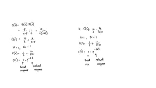
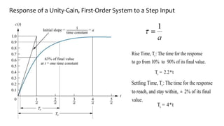
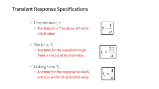
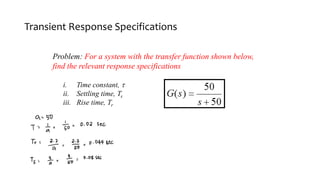
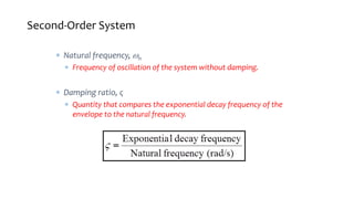
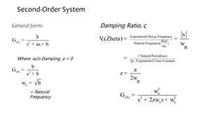
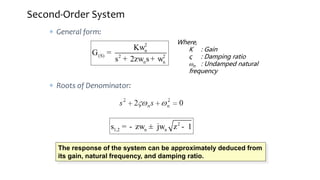
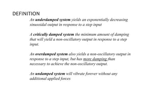
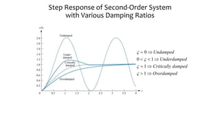
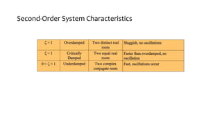
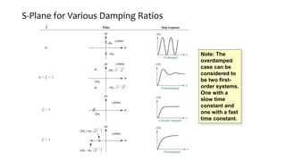
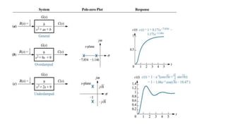
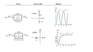
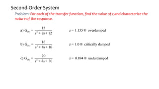
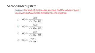
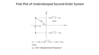
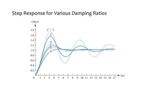
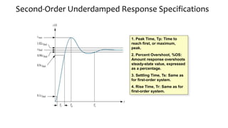
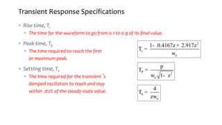
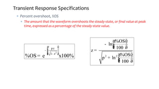
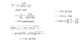
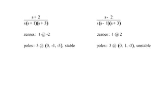
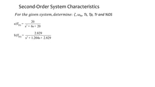
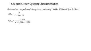
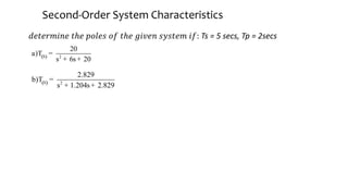
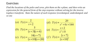
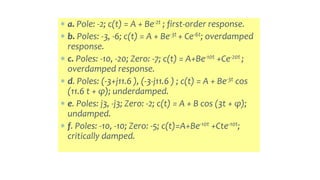
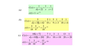
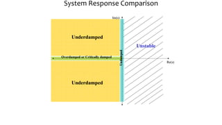
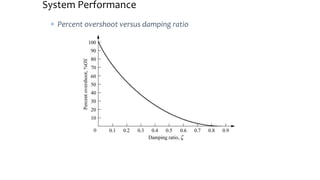
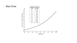
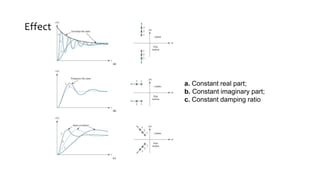
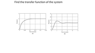
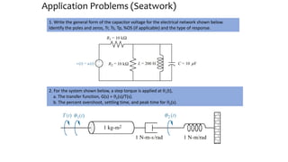
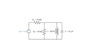
• Effect of Poles & Zeros on Time Response
• First-Order Systems: Gain/Time-Constant Format
• Second-Order Systems:
• Damping Ratio/Natural Frequency Format

Poles, Zeros & Time Response
The output response of a system is the sum of the forced response
and the natural response.
1. Forced response is also called the
steady-state response or particular solution.
2. Natural response is also called the
homogeneous response of the system

Many techniques such as solving a differential equation or
taking the inverse Laplace transform, enable us to evaluate
this output, these techniques are laborious and time-
consuming.
The concept of poles and zeros, fundamental to the analysis
and design of control systems, simplifies the evaluation of a
system’s response.

• Poles: The poles of a transfer function are those
values of s for which the function is undefined
(becomes infinite).
• Zeros: The zeros of a transfer function are those
values of s for which the function is zero.
Note : A transfer function with n poles and m zeros is said to have (n-m)
zeros at s equals infinity.

Poles and Zeros of a First-Order System

Example of the Effect of Pole/Zero Locations
1. Input pole generates
form of forced response.
2. Transfer function pole
generates form of natural
response.
3. Real axis pole
generates exponential
character of natural
response.
4. Location of zero affects
the amplitude (magnitude
of residues) of each term
of the response.

Influence of Poles on Time Response
The output response of a system is a sum of
i. Forced response
ii. Natural response
a) System showing an input and an
output
b) Pole-zero plot of the system

c) Evolution of a
system response.
Follow the blue
arrows to see the
evolution of
system
component
generated by the
pole or zero

First-Order System
General form:
Problem: Derive the transfer function for the following circuit
1
1
)
(


RCs
s
G

First-Order System
Transient Response: Gradual change of output from initial to the desired condition.
Block diagram representation:
C(s)
R(s)
1

s
K

Where,
K : Gain
 : Time constant
By definition itself, the input to the system should be a step
function which is given by the following:

First-Order System
General form:
Output response:

a) First-order system
b) Pole plot of the
system
Effect of a real-axis pole upon
transient response

First-Order System
Problem: Find the forced and natural responses for the following
systems.

Response of a Unity-Gain, First-Order System to a Step Input
r
Rise Time, T : The time for the response
to go from 10% to 90% of its final value.
s
Settling Time, T : The time for the response
to reach, and stay within, 2% of its final
value.
±
s
T 4*
= t
r
T 2.2*
= t

Transient Response Specifications
 Time constant, 
 The time for e-at to decay 37% of its
initial value.
 Rise time, Tr
 The time for the waveform to go
from 0.1 to 0.9 of its final value.
 Settling time, Ts
 The time for the response to reach,
and stay within 2% of its final value.

Problem: For a system with the transfer function shown below,
find the relevant response specifications
i. Time constant, 
ii. Settling time, Ts
iii. Rise time, Tr

Second-Order System
 Natural frequency, n
 Frequency of oscillation of the system without damping.
 Damping ratio, ς
 Quantity that compares the exponential decay frequency of the
envelope to the natural frequency.

Second-Order System
General form:
Where: w/o Damping, a = 0
(S) 2
b
G
s as b
=
+ +
(S) 2
b
G
s b
=
+
n b
w =
= Natural
Frequency
Exponential Decay Frequency
Rad
Natural Frequency( )
sec
,(Zheta)
n
s
V = =
w
1 Natural Period(sec)
2 , Exponential Time Constant
p
=
a
2
n
z =
w
Damping Ratio, ς
2
n
(S) 2 2
n n
G
s 2 s
w
=
+ zw + w

Second-Order System
 General form:
 Roots of Denominator:
Where,
K : Gain
ς : Damping ratio
n : Undamped natural
frequency
The response of the system can be approximately deduced from
its gain, natural frequency, and damping ratio.
2
n
(S) 2 2
n n
K
G
s 2 s
w
=
+ zw + w
2
1,2 n n
s j 1
= - zw ± w z -

DEFINITION
An underdamped system yields an exponentially decreasing
sinusoidal output in response to a step input
A critically damped system the minimum amount of damping
that will yield a non-oscillatory output in response to a step
input.
An overdamped system also yields a non-oscillatory output in
response to a step input, but has more damping than
necessary to achieve the non-oscillatory output.
An undamped system will vibrate forever without any
additional applied forces

Step Response of Second-Order System
with Various Damping Ratios




 
  
 
 
0
0 1
1
1
Undamped
Underdamped
Critically damped
Overdamped

Second-Order System Characteristics

S-Plane for Various Damping Ratios
Note: The
overdamped
case can be
considered to
be two first-
order systems.
One with a
slow time
constant and
one with a fast
time constant.

Second-Order System
Problem: For each of the transfer function, find the value of ς and characterize the
nature of the response.
(S) 2
12
a) G
s 8s 12
=
+ +
(S) 2
16
b) G
s 8s 16
=
+ +
(S) 2
20
c) G
s 8s 20
=
+ +
1.155 overdamped
z = ®
1.0 critically damped
z = ®
0.894 underdamped
z = ®

Second-Order System
Problem: For each of the transfer function, find the values of ς and
n, as well as characterize the nature of the response.
a)
b)
c)
d)

Pole Plot of Underdamped Second-Order System
s j j
where
n n n d
d
1 2
2
1
,       
    
 is the "damped natural frequency".

Step Response for Various Damping Ratios

Second-Order Underdamped Response Specifications
1. Peak Time, Tp: Time to
reach first, or maximum,
peak.
2. Percent Overshoot, %OS:
Amount response overshoots
steady-state value, expressed
as a percentage.
3. Settling Time, Ts: Same as
for first-order system.
4. Rise Time, Tr: Same as for
first-order system.

 Rise time, Tr
 The time for the waveform to go from 0.1 to 0.9 of its final value.
 Peak time, Tp
 The time required to reach the first
or maximum peak.
 Settling time, Ts
 The time required for the transient’s
damped oscillation to reach and stay
within ±2% of the steady-state value.
2
r
n
1 0.4167 2.917
T
- z + z
=
w
P 2
n
T
1
p
=
w - z
S
n
4
T =
zw

 Percent overshoot, %OS
 The amount that the waveform overshoots the steady-state, or final value at peak
time, expressed as a percentage of the steady-state value.
2
1
%OS e x100%
æ ö
÷
ç pz ÷
ç ÷
- ç ÷
ç ÷
ç ÷
÷
ç - z
è ø
= 2 2
%OS
ln
100
%OS
ln
100
æ ö
÷
ç
- ÷
ç ÷
ç
è ø
z =
æ ö
÷
ç
p + ÷
ç ÷
ç
è ø

( )
S 2
3.35
T
s 2.67s 3.35
=
+ +
zeroes : none
2
1,2 n n
poles : s j 1
= - zw ± w z -
( )
a 2.67
2 2 3.35
n
0.73,underdamped
z = =
w
=
( ) ( )
2
0.73 3.35 j 3.35 0.73 1
= - ± -
( )
1.34 j 1.26j
= - ±
( )
1.34 j 1.26j
= - ±
( )
1.34 1.26
13 2
2 poles @ ,
5 25
= - ± -
æ ö
÷
ç
= - - ÷
ç ÷
ç
è ø

( )( )
s 2
s s 1 s 3
+
+ +
zeroes : 1 @ -2
( )
poles : 3 @ 0, -1, -3 , stable
( )( )
s 2
s s 1 s 3
-
- +
zeroes : 1 @ 2
( )
poles : 3 @ 0, 1, -3 , unstable

𝐹𝑜𝑟 𝑡ℎ𝑒 𝑔𝑖𝑣𝑒𝑛 𝑠𝑦𝑠𝑡𝑒𝑚, 𝑑𝑒𝑡𝑒𝑟𝑚𝑖𝑛𝑒: 𝜁, 𝜔𝑛, Ts, Tp, Tr and %OS
( )
S 2
20
a)T
s 6s 20
=
+ +
( )
S 2
2.829
b)T
s 1.204s 2.829
=
+ +

( )
S 2
20
a)T
s 6s 20
=
+ +
( )
S 2
2.829
b)T
s 1.204s 2.829
=
+ +
𝑑𝑒𝑡𝑒𝑟𝑚𝑖𝑛𝑒 𝑡ℎ𝑒 𝑝𝑜𝑙𝑒𝑠 𝑜𝑓 𝑡ℎ𝑒 𝑔𝑖𝑣𝑒𝑛 𝑠𝑦𝑠𝑡𝑒𝑚 𝑖𝑓: %OS = 15% and Tp = 0.25secs

( )
S 2
20
a)T
s 6s 20
=
+ +
( )
S 2
2.829
b)T
s 1.204s 2.829
=
+ +
𝑑𝑒𝑡𝑒𝑟𝑚𝑖𝑛𝑒 𝑡ℎ𝑒 𝑝𝑜𝑙𝑒𝑠 𝑜𝑓 𝑡ℎ𝑒 𝑔𝑖𝑣𝑒𝑛 𝑠𝑦𝑠𝑡𝑒𝑚 𝑖𝑓: Ts = 5 secs, Tp = 2secs

Exercises
Find the locations of the poles and zeros, plot them on the s-plane, and then write an
expression for the general form of the step response without solving for the inverse
Laplace transform. State the nature of each response (overdamped, underdamped, and
so on)

 a. Pole: -2; c(t) = A + Be-2t ; first-order response.
 b. Poles: -3, -6; c(t) = A + Be-3t + Ce-6t; overdamped
response.
 c. Poles: -10, -20; Zero: -7; c(t) = A+Be-10t +Ce-20t ;
overdamped response.
 d. Poles: (-3+j11.6 ), (-3-j11.6 ) ; c(t) = A + Be-3t cos
(11.6 t + φ); underdamped.
 e. Poles: j3, -j3; Zero: -2; c(t) = A + B cos (3t + φ);
undamped.
 f. Poles: -10, -10; Zero: -5; c(t)=A+Be-10t +Cte-10t;
critically damped.

 
t
e
t
c
s
s
s
s
s
C
2
1
)
(
2
1
1
2
1
)
(








(a)
(b)
  
t
t
e
e
t
c
s
s
s
s
s
s
s
C
6
3
18
5
9
5
18
5
)
(
6
1
18
5
3
1
9
5
1
18
5
6
3
5
)
(













 
  
t
t
e
e
t
c
s
s
s
s
s
s
s
s
C
20
10
20
13
10
3
20
7
)
(
20
1
20
13
10
1
10
3
1
20
7
20
10
7
10
)
(














(c)

System Performance
 Percent overshoot versus damping ratio

Effect of Pole Locations
a. Constant real part;
b. Constant imaginary part;
c. Constant damping ratio

Find the transfer function of the system

Application Problems (Seatwork)
1. Write the general form of the capacitor voltage for the electrical network shown below.
Identify the poles and zeros, Tr, Ts, Tp, %OS (if applicable) and the type of response.
2. For the system shown below, a step torque is applied at q1(t),
a. The transfer function, G(s) = q2(s)/T(s).
b. The percent overshoot, settling time, and peak time for q2(s).

Time-Response Lecture

Recommended

Recommended

More Related Content

Similar to Time-Response Lecture

Similar to Time-Response Lecture (20)

Recently uploaded

Recently uploaded (20)

Time-Response Lecture