This document analyzes and models a rotational mechanical system to determine its time domain characteristics. The system is modeled using a second-order differential equation and Laplace transform. MATLAB is used to verify results and simulate the system. Key findings include: 1) The system has poles at -8 ± j20, a damping ratio of 0.3714, and 28.46% overshoot. 2) The impulse and step responses are determined and match simulations in MATLAB. 3) A state space model is developed using A, B, C, and D matrices to reduce the system to first-order equations.

1. 2015
PennState Harrisburg
Chad RyanWeiss
Mireille Mballa
CONTROL SYSTEMS LAB # 3
Rotational SystemCharacteristics

2. 1 | P a g e
Table of Contents
Category Page(s)
Objectives 2
Methods 2 – 7
Analysis 8 – 13
Design 13 – 17
Conclusion 18
References 19
Appendix 19

3. 2 | P a g e
Objectives
The objective of thislabisto analyze andmodel arotational mechanical system,tofinditstime domain
characteristics andto record itsresponse withrespecttovariousinputs. Alsoincludessome design.
The systembeinganalyzedisshowninFig.1. We assume the systemtobe weightless andinputTto act
as a stepfunction. We also considerangulardisplacementandangularaccelerationtobe the two
outputsof the system. (Assumenoinitial conditionsforthe system)
Methods
Part1 – TransferFunction
To beginouranalysis, we firstwrite the second-orderdifferentialequationthatmodelsthe system.
𝐽𝜃̈ + 𝐷𝜃̇ + 𝐾𝜃 = 𝑇
Furthermore,we take the Laplace transformationof (1) towrite itinterms of itsfrequency content.
𝐽𝑠2 𝜃( 𝑠) + 𝐷𝑠𝜃( 𝑠) + 𝐾𝜃(𝑠) = 𝑇(𝑠)
Withequation(2),the transferfunction becomes:
𝜃(𝑠)
𝑇(𝑠)
=
1
𝐽𝑠2+𝐷𝑠+𝐾
Rewriting(3) instandardformand plugginginnumbersgives:
𝜃(𝑠)
𝑇(𝑠)
=
1
𝐽⁄
𝑠2 +
𝐷
𝐽
𝑠+
𝐾
𝐽
=
0.5
𝑠2+16𝑠+464
= 𝐻(𝑠)
Fig. 1: Model of a Rotational Mechanical System
SystemParameters
 𝐽 = 2 (N-m-s2
/rad)
 𝐷 = 32 (N-m-s/rad)
 𝐾 = 928 (N-m/rad)
 𝑇 = 100 (N-m)
(1)
(2)
(3)
(4)

4. 3 | P a g e
Part2 – SystemCharacteristics
Nowthat (4) hasbeen discovered,we mayfindthe following systemcharacteristics:
 P (poles)&Z(zeros)
 𝜔 𝑛 (undampednatural frequency)
 𝜔 𝑑 (dampedfrequency)
 𝜏 (time constant)
 𝑡 𝑠 (settlingtime)
 𝑡 𝑝 (peaktime)
 𝜁 (dampingratio)
 𝑡 𝑟 (rise time)
 %𝑂𝑆 (percentovershoot)
To findthe poleswe lookatthe denominatorof ourtransferfunction andcomplete the square:
𝑠2 + 16𝑠 + 464 → (𝑠 + 8)2 + 400
Therefore the polesare:
𝑃 = −8 ± 𝑗20
The remainingsystemcharacteristicsare determinedasfollows:
𝜔 𝑛 = √464
𝜔 𝑑 = ±20
𝜏 = 0.125
𝑡 𝑠 = 0.5
𝑡 𝑝 = 0.157
𝜁 = 0.3714
Table1: Determining System Characteristics
(5)
(6)
If the polesare of form:
𝑃 = 𝑥 ± 𝑗𝑦
The transferfunctionsof form:
𝐻( 𝑠) =
1
𝑎 𝑠2 +𝑏𝑠+𝑐
The systemcharacteristicsare then:
𝜔 𝑛 = √ 𝑐
𝜔 𝑑 = ±𝑦
𝜏 = │
1
𝑥
│
𝑡 𝑠 = 4𝜏
𝑡 𝑝 =
𝜋
𝜔 𝑑
𝜁 =
𝑥
−𝜔 𝑛
(“a” must be equal to 1)
(7)
(8)
(9)
(10)
(11)
(12)

5. 4 | P a g e
Table 3: Laplace Transformations of the Unit Impulse and Decaying Sine Functions
Table 2: Determining Rise Time
To calculate the rise time,we have touse Table 2:
The final systemcharacteristicis%OS(percent overshoot);tocalculate thiswe use:
𝜁 =
−ln(
%𝑂𝑆
100
)
√(𝜋2 + 𝑙𝑛2(
%𝑂𝑆
100
)
Solving(14) for %OS gives,
%𝑂𝑆 = 28.46% 𝑜𝑟 0.2846
Part3 – ImpulseResponse
Calculatingthe impulseresponse isassimple asconvertingourequation(4) tothe time domain. Todo
so,we use Table 3:
Since the dampingratioliesinbetween0.4and 0.3, we must
extrapolate the righthandcolumnvalue throughaprocess
calledlinearinterpolation. Inourcase, the dampingratiois
approximately71.4 percentof the wayfrom 0.3 to 0.4, hence
our equationbecomes:
(1.463 − 1.321) ∗ 0.714 + 1.321 = 1.422 = 𝜔 𝑛 𝑡 𝑟
Therefore,
𝑡 𝑟 = 0.066 (13)
(14)
(15)

6. 5 | P a g e
Table 4: Laplace Transformations of the Unit Step and Generic Oscillatory Decaying Functions
By takinga lookat (4) and (5),we see that all we needtoacquire the desiredform(inTable 3) isa 20 in
the numerator;therefore we performthe followingmanipulations:
0.5
𝑠2+16𝑠+464
→
40
40
∗
0.5
𝑠2+16𝑠+64+464−64
→
1
40
∗
20
(𝑠+8)2+202
Using(16) inconjunctionwithTable 3, the impulse response of the systemis,
𝜃( 𝑡) =
𝑒−8𝑡sin(20𝑡)
40
Equation(17) isa representationof how thisparticularrotational mechanical systembehaveswhena
unitimpulse torque isapplied.
Part4 – Step Response
Findingthe stepresponse requiresthatwe convertourtransferfunctiontothe time domainusingTable
4. To do so however,the transferfunctionof the systemmustbe directlyinfluencedbyastepresponse.
Since addinginthe time domainequatestomultiplyinginthe frequencydomain,togetthe step
response of the system,we simplymultiplythe transferfunctionbythe unitinputstep(T).
0.5
𝑠2+16𝑠+464
∗
100
𝑠
=
50
𝑠∗[(𝑠+8)2+202]
To findthe valuesthatwe needforthe equationsinTable 4, we mustexpand(18) througha process
calledpartial fractionexpansion. Thisallowsustodetermine the coefficients thatcharacterize our
system’sstepresponse.
𝐴
𝑠
+
𝐵𝑠 + 𝐶
(𝑠 + 8)2 + 202
Usingthe brute force method,
𝐴𝑠2 + 𝐴 ∗ 16𝑠 + 𝐴 ∗ 464 + 𝐵𝑠2 + 𝐶𝑠 = 50
(16)
(17)
(18)
(19)
(20)

7. 6 | P a g e
464 ∗ 𝐴 = 50 → 𝐴 = 0.10776
𝐴𝑠2 + 𝐵𝑠2 = 0 → −𝐴 = 𝐵 = −0.10776
16𝑠 ∗ 𝐴 + 𝐶𝑠 = 0 → −16𝐴 = 𝐶 = −1.7241
Equation(19) isthe general expandedformof (18). Knowingthat 𝑎 = 8 and 𝜔 𝑑 = 20 fromequation
(19) and Table 4, alongwiththe resultsfrom(20-23), the stepresponse becomes:
𝜃( 𝑡) = 0.10776 + 𝑒−8𝑡[−0.10776 ∗ cos(20𝑡) − 0.0431 ∗ sin(20𝑡)]
Part5 – StateSpaceModel
In orderto reduce the second-ordersystemdowntoa first-ordersystemof linearequations,we must
construct the state space model of the system.
To begin,we declare ourstate variables:
𝑞1 = 𝜃
𝑞2 = 𝜃̇
Therefore,equation(1) becomes:
𝐽𝑞̇2 + 𝐷𝑞2 + 𝐾𝑞1 = 𝑇
From equations(25-27),we can see that,
𝑞̇1 = 𝑞2
𝑞̇2 =
𝑇 − 𝐾𝑞1 − 𝐷𝑞2
𝐽
Now,before we beginconstructingoursystemmatrices,we mustfirstwrite outthe equationsforthe
system’soutputs.
Knowingthatour outputsinclude the angulardisplacement (𝜃) andangularacceleration (𝜃̈),the
system’soutputequationsbecome:
𝑦1 = 𝑞1
𝑦2 = 𝑞̇2
Withequations(25-31),we may begintoconstruct our A,B, C and D matrices.
(21)
(22)
(23)
(24)
(25)
(26)
(27)
(28)
(29)
(30)
(31)

8. 7 | P a g e
Our A matrix isdefinedasthe systemmatrix andrelatesthe state variablestothe derivativesof the
state variable. The equationsusedtofill the A matrix are shownin(28) and(29).
A becomes:
𝐴 = [
0 1
−
𝐾
𝐽
−
𝐷
𝐽
] = [
0 1
−464 −16
]
Our B matrix isdefinedasthe matrix thatrelatesthe state variablesof the systemtothe inputof the
system. The equationsusedtofill the Bmatrix are alsoshown in(28) and(29).
B becomes:
𝐵 = [
0
1
𝐽
] = [
0
0.5
]
Our C matrix isdefinedasthe matrix thatrelatesthe system’sstate variablestothe outputof the
system. The equationsusedtofill the Cmatrix are shownin(30) and (31).
C becomes:
𝐶 = [
1 0
−
𝐾
𝐽
−
𝐷
𝐽
] = [
0 1
−464 −16
]
Our D matrix isdefinedasthe matrix thatrelatesthe outputsof the systemto itsgiveninput. The
equationsusedtofill the Dmatrix are also giveninequations(30) and(31).
D becomes:
𝐷 = [
0
1
𝐽
] = [
0
0.5
]
Withequations(32-35),we may constructour state space representationof the system.
The state space model becomes:
[
𝑞̇1
𝑞̇2
] = 𝐴 ∗ [
𝑞1
𝑞2
] + 𝐵 ∗ 𝑇
[
𝑦1
𝑦2
] = 𝐶 ∗ [
𝑞1
𝑞2
] + 𝐷 ∗ 𝑇
Withnumbers,
[
𝑞̇1
𝑞̇2
] = [
0 1
−464 −16
] [
𝑞1
𝑞2
] + [
0
0.5
] 𝑇
[
𝑦1
𝑦2
] = [
1 0
−464 −16
][
𝑞1
𝑞2
] + [
0
0.5
] 𝑇
(32)
(33)
(34)
(35)
(38)
(39)
(36)
(37)

9. 8 | P a g e
Analysis
Nowthat we’ve gone throughthe methods,we canbegintouse computational engineslikeMATLABto
verifyourresults. The MATLAB script(shownbelow)willallow ustodeterminethe following:
 PolesandZeros
 Impulse andStepResponse
 TransferFunctionMatrix
The great thingaboutMATLAB isthat, aside fromallowingustobreeze throughcalculations,italso
allowsusto visualizeourresultsbygeneratingplots.
As youcan see fromFig.2, MATLAB providesveryuseful toolsforanalyzingvarioussystems. Bysimply
definingoursystemtransferfunctionandglobal variables,we were able touse MATLAB’spzmap
functiontocreate a visual representationof the polesandzerosof the system. Asyoucan see,they
occur at -8±j20, whichhappenstobe consistentwithwhatwe foundearlierinequation(6).
Furthermore,thisfunctionalsogivesusthe valuesforthe dampingratioandpercentovershootof the
system,which alsohappenstobe consistentwith the resultsthatwe foundearlier. See (12) and (15).
Applyingthe scriptandsolvingforthe impulseresponsegivesus:
Figure 2: Pole-Zero Map of System H
(40)

10. 9 | P a g e
Similarly forthe stepresponse,
Similarly forthe transferfunction matrix,
So justby usingthe MATLAB script (shownabove),we were able tocome upwithquickanswersto
relativelydifficultcalculationsforoursystem.
We can alsouse an extensionof MATLABcalledSimulinktomodel oursystemandobserve the outputs.
Figure 3: Transfer Function Block Diagram Model of a Rotational Mechanical System
(41)
(42)
The blockdiagram showninFig.3 isa
basicmodel of our rotational
mechanical system. Asyoucan see,
there are two inputsinthismodel and
each feedsintothe transferfunction
or outputvs. inputequationof the
system. Atthe opposite endof the
model we place multiple scopesto
observe variousoutputs. See Fig.4-6
Figure 4: Step Input versus System Output

11. 10 | P a g e
Figure 5: Impulse Input versus System Output
If we delve deeperandexamine ouroutputsmore closely,we canextractsome of the system
parametersrightfromthe simulation.
Figure 6: System Outputs

12. 11 | P a g e
If you lookat Fig.6, you will immediatelynotice thatthe rise timesare notconsistent. Anexplanation
mightbe that the amplitude of the impulse hasadirectcorrelationtothe rise time of the impulse
output. Aside fromthattinymismatch,the simulatedoutputs,more orless,give usresultsthatare
similartothe oneswe derivedfromourmethods. InFig.6 you can see that the settlingtime,peaktime
and percentovershootare verysimilartothe valueswe calculatedinequations(10),(11) and(15). You
can tell thatthis simulationisfairlyaccurate due tothe final value of the stepresponse.
Anotherblockdiagramthatcan be used to simulate oursystem’sresponse isbasedoff equation(29).
Fig.7 isa purelymathematical representationof oursystem. Thismodel will provide the same exact
resultsasthe transferfunctionblockdiagramshowninFig.3. Forcomparison,see Fig.6 & 8.
The main advantage of the mathematical blockdiagramoverthe transferfunctionblockdiagramisthat
if we wantedto take a lookat the angularaccelerationof oursystem, all we needdoisadjustthe scope
like so: (NextPage)
Figure 7: Mathematical Block Diagram for a Rotational Mechanical System
Figure 8: Rotational Mechanical System Angular Displacement Step Response

13. 12 | P a g e
Figure 11: Transfer Function Block Diagram with Additional Outputs
The resultwill be the angularaccelerationof the system:
Figure 10: Rotational Mechanical System Angular Acceleration Step Response from Math BasedBlock Diagram
In orderto viewthe angularaccelerationfromthe transferfunctionblockdiagram, more components
wouldbe necessary.
Figure 9: Mathematical Block Diagram for a Rotational Mechanical System – Scope at Different Output

14. 13 | P a g e
As youcan see fromFig.12, the angular accelerationisnodifferentthanthe one simulatedinFig.10.
Despite havingcompletelydifferentstructures, the blockdiagramrepresentationsof oursystem,
(showninFigs.9 & 11) provide uswithidentical results.
Design
Our nextobjectiveistoredesignthe systemsothatthe dampingratioζ is equal to0.707.
To accomplishthis,ournewsystemparametersbecome:
Part1 – TransferFunction
Therefore,ourtransferfunction becomes:
𝜃(𝑠)
𝑇(𝑠)
=
1
𝐽⁄
𝑠2 +
𝐷
𝐽
𝑠+
𝐾
𝐽
=
0.5
𝑠2+30𝑠+450
= 𝐻(𝑠)
WithPoles:
𝑃 = −15 ± 𝑗15
Figure 12: Rotational Mechanical System Angular Acceleration Step Response from Transfer Function Block Diagram
SystemParameters
 𝐽 = 2 (N-m-s2
/rad)
 𝐷 = 60 (N-m-s/rad)
 𝐾 = 900 (N-m/rad)
 𝑇 = 100 (N-m)
(43)
(44)

15. 14 | P a g e
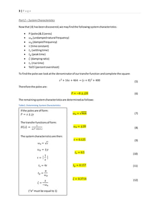
Part2 – SystemCharacteristics
Using(43) and(44) withTables1 and2, alongwithequation(14),our systemcharacteristicsbecome:
𝜔 𝑛 = √450
𝜔 𝑑 = ±15
𝜏 = 0.067
𝑡 𝑠 = 0.267
𝑡 𝑝 = 0.209
𝜁 = 0.707
𝑡 𝑟 = 0.100
%𝑂𝑆 = 4.32%
Part3 – ImpulseResponse
By takinga lookat (43), we see that all we need todo to acquire the desiredform inTable 3 isa 15 in
the numerator;therefore we performthe followingmanipulationstoacquire the impulse response:
0.5
𝑠2+30𝑠+450
→
30
30
∗
0.5
𝑠2+30𝑠+225+450−225
→
1
30
∗
15
(𝑠+15)2+152
Using(53) inconjunctionwithTable 3,the impulse response of the systembecomes,
𝜃( 𝑡) =
𝑒−15𝑡sin(15𝑡)
30
Part4 – Step Response
To get the step response of the system,we simplymultiplythe transferfunctionbythe unitinputstep.
0.5
𝑠2+30𝑠+450
∗
100
𝑠
=
50
𝑠∗[(𝑠+15)2+152]
Then,we mustexpand(55) througha processcalledpartial fractionexpansion,allowingustodetermine
the coefficientsthatcharacterize oursystem’sstepresponse.
𝐴
𝑠
+
𝐵𝑠 + 𝐶
(𝑠 + 15)2 + 152
Usingthe brute force method,
𝐴𝑠2 + 𝐴 ∗ 30𝑠 + 𝐴 ∗ 450 + 𝐵𝑠2 + 𝐶𝑠 = 50
(46)
(47)
(48)
(49)
(50)
(45)
(51)
(52)
(53)
(54)
(56)
(57)
(55)

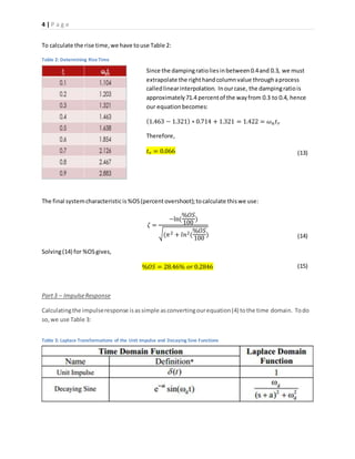
16. 15 | P a g e
450 ∗ 𝐴 = 50 → 𝐴 = 0.111
𝐴𝑠2 + 𝐵𝑠2 = 0 → −𝐴 = 𝐵 = −0.111
30𝑠 ∗ 𝐴 + 𝐶𝑠 = 0 → −30𝐴 = 𝐶 = −3.33
Equation(56) isthe general expandedformof (55).Knowingthat 𝑎 = 15 and 𝜔 𝑑 = 15 fromequation
(56) and Table 4, alongwiththe resultsfrom(58-60), the stepresponse becomes:
𝜃( 𝑡) = 0.111 − 𝑒−15𝑡[0.111 ∗ cos(15𝑡) + 0.333 ∗ sin(15𝑡)]
Part5 – Analysis
By makingthe necessarychangestothe followingscript,we canverifythe datafor our new system.
As youcan see by lookingatFig.13, the polesoccurat -15±j15 as expected. Also,youcansee that the
dampingratiois0.707 and the percentovershootis4.32%, all of whichhappentobe consistentwiththe
calculatedvaluesobtainedinequations(44),(50) and (52).
Applyingthe scriptandsolvingforthe impulseresponsegivesus:
(58)
(59)
(60)
(61)
Figure 13: Pole-Zero Map of the Newly DesignedSystem
(62)

17. 16 | P a g e
Similarlyforthe stepresponse:
Now, reconstructingthe blockmodel diagramandmakingthe necessary changestothe centertransfer
functions allowsusto viewthe outputof ournewlydesigned systemlike before.
Figure 14: Transfer Function Block Diagram for the Redesigned System
(63)
Figure 15: Step Response of the Newly Designed System

18. 17 | P a g e
As youcan see inFig.15, the stepresponse of ournewlydesignedsystemissimilartothe time domain
equationthatwe calculatedinequation(61). Some noticeable, similarcharacteristics obtainedvia
inspection include:
1) Steady-State value of approximately0.111
2) Percent-Overshootabout four, fivepercent
3) Rise-Time equalto0.1 s
4) Settling-Time about0.3s and
5) Peak-Time equal to0.2s
Comparingthe data fromFig.15 to the stepresponse andcharacteristicsof the systemprove thatour
calculationsare accurate and that our systemmodel iscorrect.
Figure 16: Impulse Response of the Newly Designed System
The same thingcan be saidabout the impulse response. Similartothe time domainequationfoundin
equation(54),Fig.16 showsthatthe systemhasa final steady-statevalue of zeroandsettlesaround0.3
seconds. Typically,the impulseresponse isnot a useful indicatorforthe rise time,peaktime orpercent
overshootfora givensystem. Thisisdue tothe factthat impulsesvarywhenitcomestodurationor
pulse width. If we adjustedthe pulse widthtogive similarcharacteristicstothatof our stepresponse,it
wouldbe an accurate representation;however,since the systemcharacteristicsare all thatwe care
aboutand natural impulsesare rarelyevervariable,we justlookatthe system’sstepresponseforthe
purposesof thislaboratory exercise.

19. 18 | P a g e
Conclusion
In thislab,our twooutputswere definedasthe angulardisplacement (𝜃) andthe angularacceleration
(𝜃̈) of a rotatingmass centeredbetweenafixedspringanddamper. The systemwasassumedtobe
frictionless andwithoutinitial conditions.
Giventhe systemparameters,we were askedtofindthe definingcharacteristicsof this system;
characteristics suchas the transientandsteady-state response of the system,aswell asthe system’s
impulse andstepresponses. Forthatreason, MATLAB and Simulinkwere usedtosimulatethe output
behaviorof the system(s). Notonlythat,MATLAB wasusedto verifythe system(s) characteristics,the
polesandzeros,andthe transferfunctionmatrix;however,itwasnohelpinassemblingthe state-space
representationof oursystemand no matterwhatwe tried,we couldnot getour hand calculated sine
termcoefficients (forbothof ourstepresponses) tomatchthe resultsobtainedviaMATLAB. See
equations(24) and(41) as well asequations(61) and(63). Otherthan that,MATLAB provideduswith
identical resultsforourimpulse response anditgave uswhat we expectedwhenitcomestopolesand
zerosby generatingpole-zeroplotsforeachone of our systems.
The main disadvantage of usingacomputational engine suchasMATLAB isthat it doesnotshow you
howit came to its final conclusion;therefore, thereare nopersonal explanationsprovidedwhenever
our owncalculationsturnoutto have eventhe slightestdifference. Sometimes ithelpstolookatthe
answeras mistakesare made clear;however, oftentimes,MATLABprovideszero clarity. Despite this
majordisadvantage,MATLABscriptingallowedustoverifymostof our resultswhile allowingusto
bypasshoursof rigoroushandcalculationsandthatis one of its mostredeemingqualities.
Aside fromusingMATLABin calculatingsystemcharacteristics,we alsousedSimulinktoconstruct
logical blockdiagramsthatservedusina varietyof ways. MATLAB’sSimulinkallowedustotake our
system,reconstructitona computer,testitagainstmultiple inputsandobserve the outputs. Inthislab,
there were twomethodsinconstructingthe interactivemodelsthatrepresentedoursystem(s);
althougheachmethod providedidentical outputs,therewere noticeable advantagesanddisadvantages
for eachone. The transferfunctionblock diagrams,showninFigs.(3) and(14), proved beneficial
wheneverwe neededtoviewthe stepandimpulse responsessimultaneously;however,itdidnotallow
us to viewthe angularaccelerationoutput,northe angularvelocity forthatreason,withoutadding
more componentstothe model.See Fig. (11).Forthe state-space (mathematical) blockdiagram, itwas
advantageousbecause itwascomprehensive,meaningthatthe angulardisplacement,velocityand
accelerationwere all inclusive. Thus,if we wantedtoview anyof the outputs,all we hadto do was
move our scope fromone spotto the other,withoutaddingany additionalcomponents. Itsdownfall
howevercame aboutonce we realizedthatitwasnot possible toview the stepresponse andimpulse
response simultaneouslywithoutaddingmore components. See Figs.(7) and(9).
Finally,we were askedtoredesignoursystemsothatthe systemparametersyielded adampingratioof
0.707. The mainnoticeable differencesobservedbetweenouroriginal systemandourredesigned
systemwere 1) the overshootwassignificantlyreduced, 2) the steady –state valueswere slightly
decreasedand 3) the settlingtimesweremuchshorterindicatingthatthe doublingof the dampinghad
a major influence onthe redesigned systemandthe springconstant,notsomuch.

20. 19 | P a g e
References
http://www.engr.uky.edu/~donohue/ee211/ee211_9.pdf [1]
Appendix
Tables
Name Page(s)
Table 1: DeterminingSystemCharacteristics 3
Table 2: DeterminingRise Time 4
Table 3: Laplace Transformationsof the UnitImpulse andDecayingSine Functions 4
Table 4: Laplace Transformationsof the UnitStepand GenericOscillatoryDecayingFunctions 5
Figures
Name Page(s)
Figure 1: Model of a Rotational Mechanical System 2
Figure 2: Pole-ZeroMapof SystemH 8
Figure 3: TransferFunctionBlockDiagramModel of a Rotational Mechanical System 9
Figure 4: StepInputversusSystemOutput 9
Figure 5: Impulse InputversusSystemOutput 10
Figure 6: SystemOutputs 10
Figure 7: Mathematical BlockDiagramfor a Rotational Mechanical System 11
Figure 8: Rotational Mechanical SystemAngularDisplacementStepResponse 11
Figure 9: Mathematical BlockDiagram – Scope at DifferentOutput 12
Figure 10: AngularAccelerationStepResponse fromMathBasedBlockDiagram 12
Figure 11: TransferFunctionBlockDiagramwithAdditionalOutputs 12
Figure 12: AngularAccelerationStepResponse fromTransferFunctionBlockDiagram 13
Figure 13: Pole-ZeroMapof the NewlyDesignedSystem 15
Figure 14: TransferFunctionBlockDiagramforthe RedesignedSystem 16
Figure 15: StepResponse of the NewlyDesignedSystem 16
Figure 16: Impulse Response of the NewlyDesignedSystem 17