Downloaded 247 times


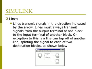
![SISOTOOL
to make the plant model and start the
SISO design tool, at the MATLAB prompt
type
>>Gp = tf(1,[1 7 10 0])
>>sisotool
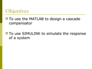
To add a damping ratio line,
Left click + design constrain + new
Constraint type: damping ratio
Damping ratio > 0.6
](https://image.slidesharecdn.com/controlchap9-131231194056-phpapp01/85/Control-chap9-5-320.jpg)

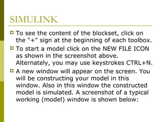

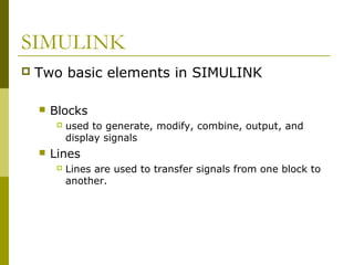
![SIMULINK
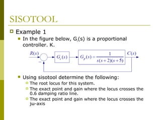
Modifying blocks
A block can be modified by double-clicking on
it.
[1] → 1
[ 1 1] → s + 1
[ 1 2 1] → s 2 + 2s + 1
[ 1 2 0] → s 2 + 2 s + 0](https://image.slidesharecdn.com/controlchap9-131231194056-phpapp01/85/Control-chap9-13-320.jpg)


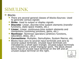
![SIMULINK
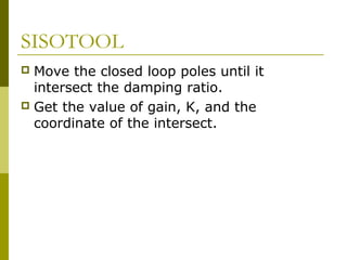
Modify blocks
Follow these steps to properly modify the blocks in
your model.Double-click your Sum block. Since you
will want the second input to be subtracted, enter
+- into the list of signs field. Close the dialog box.
Double-click your Gain block. Change the gain to
2.5 and close the dialog box.
Double-click the leftmost Transfer Function block.
Change the numerator to [1 2] and the
denominator to [1 0]. Close the dialog box.
Double-click the rightmost Transfer Function block.
Leave the numerator [1], but change the
denominator to [1 2 4]. Close the dialog box. Your
model should appear as:](https://image.slidesharecdn.com/controlchap9-131231194056-phpapp01/85/Control-chap9-18-320.jpg)


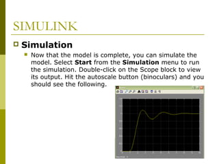

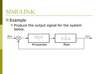
The document discusses using MATLAB and Simulink to design and simulate control systems. It provides instructions on how to: 1) Use the sisotool in MATLAB to design a cascade compensator and determine the root locus, gain where it intersects a 0.6 damping ratio line, and where it intersects the jω-axis. 2) Build models in Simulink by adding blocks like sources, sinks, transfers functions, gains and connecting them. 3) Modify block parameters and simulate the model response in the scope to analyze system performance.