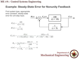
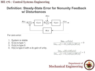
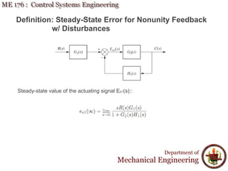
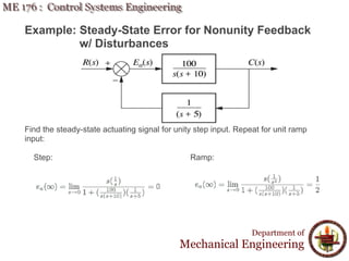
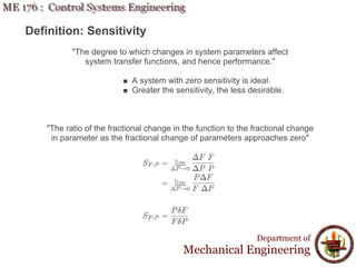
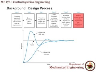
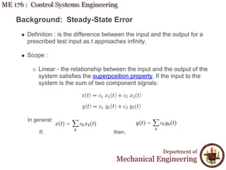
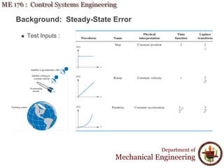
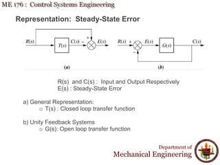
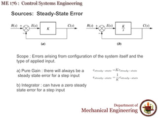
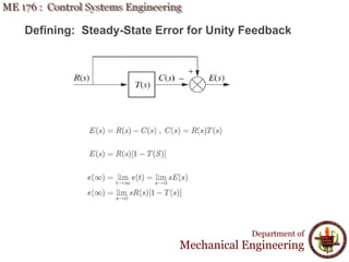
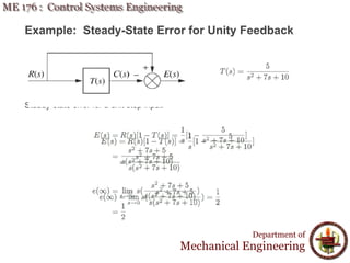
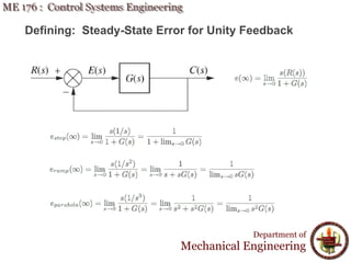
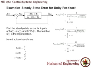
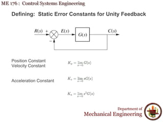
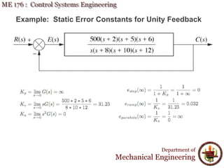
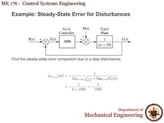
This document discusses steady-state error in control systems. It defines steady-state error and describes how it arises from system configuration and input type. Examples are provided to illustrate calculating steady-state error for various system types and inputs, including step, ramp, and disturbances. Sensitivity analysis is also introduced to analyze how changes in system parameters affect steady-state error.

1. ME 176
Control Systems Engineering
Steady-State Errors
Department of
Mechanical Engineering

2. Background: Design Process
Department of
Mechanical Engineering

3. Background: Analysis & Design Objectives
"Analysis is the process by which a system's performance is determined."
"Design is the process by which a systems performance is created or changed."
Transient Response Steady State Error
Steady State Response Stability
Department of
Mechanical Engineering

4. Background: Steady-State Error
Definition : is the difference between the input and the output for a
prescribed test input as t approaches infinity.
Scope :
Linear - the relationship between the input and the output of the
system satisfies the superposition property. If the input to the
system is the sum of two component signals:
In general:
If, then,
Department of
Mechanical Engineering

5. Background: Steady-State Error
Scope :
Time invariant systems - are systems that can be modeled with a
transfer function that is not a function of time except expressed
by the input and output.
"Meaning, that whether we apply an input to the system now or T
seconds from now, the output will be identical, except for a time delay
of the T seconds. If the output due to input x (t ) is y (t ), then the output
due to input x (t − T ) is y (t − T ). More specifically, an input affected by
a time delay should effect a corresponding time delay in the output,
hence time-invariant."
STABLE
Department of
Mechanical Engineering

6. Background: Steady-State Error
Test Inputs :
Department of
Mechanical Engineering

7. Evaluating: Steady-State Error
1. Step Input:
Output 1 : No
Steady-State Error
Output 2 : Constant
Steady-State Error
of e2
2. Ramp Input
Output 1 : No
Steady-State Error
Output 2 : Constant
Steady-State Error
of e2
Output 3 : Infinite
Steady-State Error
Department of
Mechanical Engineering

8. Representation: Steady-State Error
R(s) and C(s) : Input and Output Respectively
E(s) : Steady-State Error
a) General Representation:
T(s) : Closed loop transfer function
b) Unity Feedback Systems
G(s): Open loop transfer function
Department of
Mechanical Engineering

9. Sources: Steady-State Error
Scope : Errors arising from configuration of the system itself and the
type of applied input.
a) Pure Gain : there will always be a
steady state error for a step input
b) Integrator : can have a zero steady
state error for a step input
Department of
Mechanical Engineering

10. Defining: Steady-State Error for Unity Feedback
Department of
Mechanical Engineering

11. Example: Steady-State Error for Unity Feedback
Steady-state error for a unit step input:
Department of
Mechanical Engineering

12. Defining: Steady-State Error for Unity Feedback
Department of
Mechanical Engineering

13. Example: Steady-State Error for Unity Feedback
Find the steady-state errors for inputs
of 5u(t), 5tu(t), and 5t^2u(t). The function
u(t) is the step function.
Note Laplace transforms:
Department of
Mechanical Engineering

14. Defining: Static Error Constants for Unity Feedback
Position Constant
Velocity Constant
Acceleration Constant
Department of
Mechanical Engineering

15. Example: Static Error Constants for Unity Feedback
Department of
Mechanical Engineering

16. Example: Static Error Constants for Unity Feedback
Department of
Mechanical Engineering

17. Example: Static Error Constants for Unity Feedback
Department of
Mechanical Engineering

18. System Types for
Unity Feedback:
Given the system shown, the
"system type" is defined as the
value of "n" in the denominator;
or, equivalently the number of pure
integrations in the feedforward path.
Department of
Mechanical Engineering

19. Specifications: Steady-State Error
"Static error constants can be used to specificy the
steady-state error characteristics of a control system."
Knowing Kp = 1000 what can be learned of the system:
1. System is stable.
2. System is Type 0
3. Input Test signal is step.
4. Error per unit step:
Department of
Mechanical Engineering

20. Example: Steady-State Error Specification
Find K so that there is a 10% error in steady state.
Since system is Type 1, error stated must apply to ramp function.
Department of
Mechanical Engineering

21. Analysis: Steady-State Error for Disturbances
"Steady-state error produced by a step
function can be reduced by increasing
the gain of G1(s) or decreasing the
gain of G2(s)."
Department of
Mechanical Engineering

22. Example: Steady-State Error for Disturbances
Find the steady-state error component due to a step disturbance.
Department of
Mechanical Engineering

23. Definition: Steady-State Error for Nonunity Feedback
Move R(s) to right
of summing
junction.
Compute resulting
G(s) and H(s).
Add and subtract
unity feedback
paths.
Combine negative
feedback path to H
(s).
Combine feedback
system consisting
of G(s) and [H(s)
-1].
Department of
Mechanical Engineering

24. Example: Steady-State Error for Nonunity Feedback
Find system type, appropriate
error constant, steady-state
error for unit step input.
Department of
Mechanical Engineering

25. Definition: Steady-State Error for Nonunity Feedback
w/ Disturbances
General form: For step input and step distrubances:
Department of
Mechanical Engineering

26. Definition: Steady-State Error for Nonunity Feedback
w/ Disturbances
For zero error:
1. System is stable
2. G1(s) is type 1.
3. G2(s) is type 0.
4. H(s) is type 0 with a dc gain of unity.
Department of
Mechanical Engineering

27. Definition: Steady-State Error for Nonunity Feedback
w/ Disturbances
Steady-state value of the actuating signal Ea1(s)::
Department of
Mechanical Engineering

28. Example: Steady-State Error for Nonunity Feedback
w/ Disturbances
Find the steady-state actuating signal for unity step input. Repeat for unit ramp
input:
Step: Ramp:
Department of
Mechanical Engineering

29. Definition: Sensitivity
"The degree to which changes in system parameters affect
system transfer functions, and hence performance."
A system with zero sensitivity is ideal.
Greater the sensitivity, the less desirable.
"The ratio of the fractional change in the function to the fractional change
in parameter as the fractional change of parameters approaches zero"
Department of
Mechanical Engineering

30. Example: Sensitivity
Calculate sensitivity of the closed-loop transfer function to changes in parameter a:
Closed-loop transfer function:
Department of
Mechanical Engineering

31. Example: Sensitivity
Calculate sensitivity of the closed-loop transfer function to changes in parameter K
and a, with ramp inputs:
Department of
Mechanical Engineering