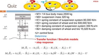
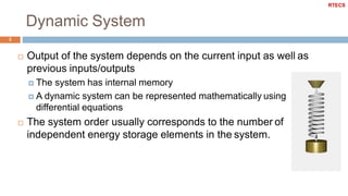
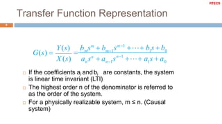
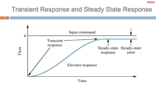
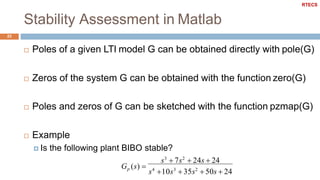
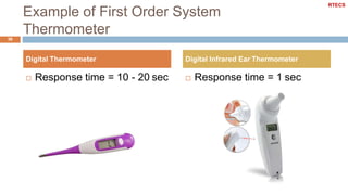
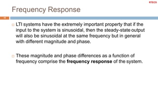
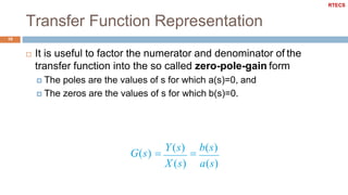
This document discusses dynamic systems and their analysis using transfer functions. It begins by defining dynamic systems as those whose output depends on both current and previous inputs/outputs. It then covers: - Transfer function representations of linear time-invariant (LTI) systems using Laplace transforms. - Key properties of transfer functions including poles, zeros and zero-pole-gain form. - MATLAB representations of transfer functions. 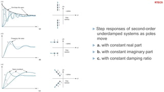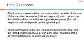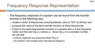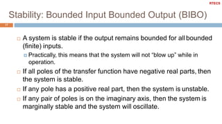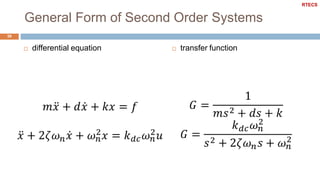It also defines important concepts for analyzing dynamic systems like time and frequency response, stability, system order, and the effects of pole locations. Specific discussions are included on analyzing first and second order systems.

1. DYNAMIC SYSTEM ANALYSIS
15-Mar-17
RTECS 2015 1
Eng. Mahmoud Hussein
RTECS

2. Dynamic System
3
 Output of the system depends on the current input as well as
previous inputs/outputs
 The system has internal memory
 A dynamic system can be represented mathematically using
differential equations
 The system order usually corresponds to the number of
independent energy storage elements in the system.
RTECS

3. Transfer Function Representation
4
 LTI systems have the extremely important property that if the
input to the system is sinusoidal, then the output will also be
sinusoidal at the same frequency but in general with different
magnitude and phase.
 These magnitude and phase differences as a function of
frequency are known as the frequency response of the
system.
RTECS

4. Transfer Function Representation
5
 Using the Laplace transform, it is possible to convert a
system's time-domain representation into a frequency-domain
output/input representation, known as the transfer function.
 In so doing, it also transforms the governing differential
equation into an algebraic equation which is often easier to
analyze.
 Frequency-domain methods are most often used for analyzing
LTI single-input/single-output (SISO)systems, e.g. those
governed by a constant coefficient differential equation
RTECS

5. Transfer Function Representation
6
 The Laplace transform of a time domain function
0
Where
s    j complex frequency variable

 st
F(s)  f (t)e dt
RTECS

6. Transfer Function Representation
7
 A transfer function is the Laplace transform of thesystem’s
differential equation with omitting initial conditions
 Hence, it is a rational function of the variable ‘s’
01nX (s) a sn
 a s
Y(s) b sm
b
G(s)  n1
n1
m m1 1 0
 a s  a
sm1
 b s b
RTECS

7. Transfer Function Representation
8
 If the coefficients ai andbi are constants, the system
is linear time invariant (LTI)
 The highest order n of the denominator is referred to
as the order of the system.
 For a physically realizable system, m ≤ n. (Causal
system)
Y(s)
nX (s) a sn
 a s
b sm
 b
G(s)  n1
n1 1 0
m m1 1 0
 a s  a
sm1
 b s  b
RTECS

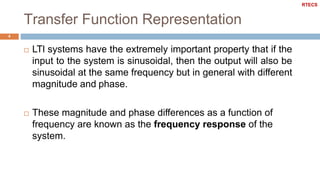
8. MATLAB Representations of Transfer Functions
9
 num=[b1,b2,. . .,bm,bm+1];
 den=[1,a1,a2,. . .,an−1, an];
 G=tf(num,den)
 Example
s4
 2s3
 3s2
 4s  5
s 5
G(s) 
RTECS

9. Transfer Function Representation
10
 It is useful to factor the numerator and denominator of the
transfer function into the so called zero-pole-gain form
 The poles are the values of s for which a(s)=0, and
 The zeros are the values of s for which b(s)=0.
G(s) 
Y(s)

b(s)
X (s) a(s)
RTECS

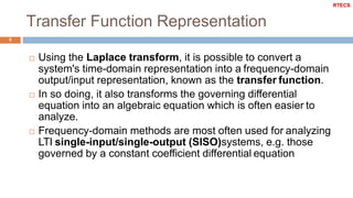
10. Zero-Pole-Gain Representation In MATLAB
11
 z=-[z1; z2; · · · ; zm];
 p=-[p1; p2; · · · ; pn];
 G=zpk(z,p,K)
 Example
s 3
(s  2)(s  4)(s  5)
 pzmap
 Plots the pole-zero map of the LTI model sys
RTECS

11. Terms and Definitions
System Analysis12
RTECS

12. Time Response
13
 The time response of a linear dynamic system consists of the sum
of the transient response (Natural response) which depends on
the initial conditions and the steady-state response (Forced
response ) which depends on the system input.
 These correspond to the free (homogeneous or zero input) and
the forced (inhomogeneous or non-zero input) solutions of the
governing differential equations respectively.
RTECS

13. Transient Response and Steady State Response
14
RTECS

14. Frequency Response
15
 LTI systems have the extremely important property that if the
input to the system is sinusoidal, then the steady-state output
will also be sinusoidal at the same frequency but in general
with different magnitude and phase.
 These magnitude and phase differences as a function of
frequency comprise the frequency response of the system.
RTECS

15. Frequency Response Representation
16
 The frequency response of a system can be found from the transfer
function in the following way:
 create a vector of frequencies (varying between zero or "DC" to infinity) and
 compute the value of the plant transfer function at those frequencies.
 If G(s) is the open-loop transfer function of a system and ω is the frequency
vector, we then plot G(j ω ) versus ω . Since G(j ω ) is a complex number,
we can plot
 both its magnitude and phase (the Bode Plot) or
 its position in the complex plane (the Nyquist Diagram).
RTECS

16. Stability: Bounded Input Bounded Output (BIBO)
17
 A system is stable if the output remains bounded for allbounded
(finite) inputs.
 Practically, this means that the system will not “blow up” while in
operation.
 If all poles of the transfer function have negative real parts, then
the system is stable.
 If any pole has a positive real part, then the system is unstable.
 If any pair of poles is on the imaginary axis, then the system is
marginally stable and the system will oscillate.
RTECS

17. Effect of Pole Location
18
 Consider the transfer function
 The impulse response will be an
exponential function
RTECS

18. Effect of Pole Location
19
 When σ > 0, the pole is located at s < 0,
 The exponential expression y(t) decays.
 Impulse response is stable.
 When σ < 0, the pole is located at s > 0,
 The exponential expression y(t) grows with time.
 Impulse response is referred to as unstable.
if   0
Im(s)
if   0
Re(s)
if   0y(t)
if   0
t
RTECS

19. Effect of Pole Location: Example
20
 Find the impulse response of H(s)
H (s)
s2
2s 1

2s 1
 3s 2 (s 1)(s  2)

1

3
s 1 s 2
1 

s 1
 
s  2

   
h(t)  L1  1  3L1 
h(t)  (et
 3e2t
)1(t) 0 1 2 3
Time (sec)
4
-0.5
0
0.5
1
1.5
2
h(t)
RTECS

20. Effect of Pole Location: Example
21
 syms s t;
 H=(2*s+1)/(s^2+3*s+2);
 h=ilaplace(H);
RTECS

21. Stability Criterion Vs. Pole Locations
Impulse Response22
Re(s)
Im(s)
y(t) y(t)
y(t)
t
t
t
y(t)
t
y(t)
t
y(t)
t
RTECS

22. Stability Assessment in Matlab
23
 Poles of a given LTI model G can be obtained directly with pole(G)
 Zeros of the system G can be obtained with the function zero(G)
 Poles and zeros of G can be sketched with the function pzmap(G)
 Example
 Is the following plant BIBO stable?
s3
 7s2
 24s  24
Gp (s) 
s4
10s3
 35s2
 50s  24
RTECS

23. System Order
24
 The order of a dynamic system is the order of the highest
derivative of its governing differential equation.
 Equivalently, it is the highest power of s in the denominator of
its transfer function.
RTECS

24. First Order Systems25
RTECS

25. General Form of First Order Systems
 differential equation  transfer function
26
RTECS

26. DC Gain
27
 The DC gain is the ratio of the magnitude of the steady-state
step response to the magnitude of the step input
 DC gain is the value of the transfer function when s=0.
 For first order systems equal to
RTECS

27. Time Constant
28
 The time constant represents the time scale for which the dynamics
of the system are significant.
 For first order systems, the time constant is the time it takes for the
system to reach 63% of the steady-state value for a step response
or to decrease to 37% of the initial value for an impulse response.
RTECS

28. Poles/Zeros of First Order Systems
29
 There is a single real pole at s = -a
 Therefore, the system is stable if a is positive and unstable if a is
negative
 There are no zeros
RTECS

29. Step Response of First-Order Systems
30
a
s(s a)
C(s)  R(s)G(s) 
c(t)  c (t)  c (t) 1 eat
f n
RTECS

30. Step Response of First-Order Systems
Time Constant31
 Time for the system output to
reach approximately 63% of its
final steady state value
 indication of system response
speed
c(t)  c (t)  c (t) 1 eat
f n
eat
 e1
0.37
t 1
a
1 0.37  0.63
a
t1
t1
a
x(t) 1 eat
RTECS

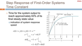
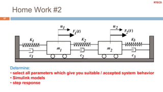
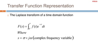
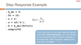
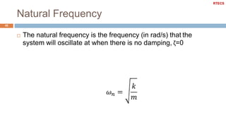
31. Step Response Example
32
 a = 5;
 num = a;
 den = [1 a];
 figure
 step(num,den);
 grid on
a
s a
G(s) 
0 0.2 0.4 0.8 1 1.2
0
0.2
0.1
0.3
0.4
0.5
0.6
0.7
0.8
0.9
1
Step Response
0.6
Time (sec)
Amplitude
RTECS

32. Step Response Example
33
 k_dc = 5;
 Tc = 10;
 u = 2;
 s = tf('s');
 G = k_dc/(Tc*s+1)
 step(u*G)
If you right click on the step response graph
and select Characteristics, you can choose
to have several system metrics overlaid on
the response: peak response, settling time,
rise time, and steady3/-1s5/t2a01t7e.
G(s) 
kdc
s 1
RTECS

33. Settling Time
34
 The settling time is the time
required for the system output to
fall within 2% percentage of the
steady state value for a step input
or equivalently to decrease to a
certain percentage of the initial
value for an impulse input.
 For first order systems, settling
time is approximately 3.9 * time
constant
RTECS

34. Rise Time
35
 The rise time is the time
required for the system output
to rise from 10% to 90% of the
final steady-state value.
 Tr = 2.2 /a
RTECS

35. Example of First Order System
Thermometer
 Response time = 10 - 20 sec  Response time = 1 sec
36
Digital Thermometer Digital Infrared Ear Thermometer
RTECS

36. Second Order Systems37
RTECS

37. Second Order Systems
38
 Second order systems are the simplest type of dynamic system
to exhibit oscillations
RTECS

38. General Form of Second Order Systems
 differential equation  transfer function
39
RTECS

39. DC Gain
40
 The DC gain is the ratio of the magnitude of the steady-state
step response to the magnitude of the step input
 DC gain is the value of the transfer function when s=0.
 For second order systems equal to
RTECS

40. Damping Ratio
41
 The damping ratio is a dimensionless quantity characterizing
the energy losses in the system due to such effects as viscous
friction or electrical resistance
RTECS

41. Natural Frequency
42
 The natural frequency is the frequency (in rad/s) that the
system will oscillate at when there is no damping, ζ=0
RTECS

42. Steady-state Value y(∞)
43
 The steady-state value of the system under the step response
is the output when t → ∞.
 Using the final value theorem
 The steady-state value of the system G can be evaluated using
the function
 K=dcgain(G)
a0
s
y()  lim sG(s)
1
s0
 G(0) 
b0
RTECS

43. Poles/Zeros of Second Order Systems
44
 The second order transfer function has two poles at
RTECS

44. Under Damped System: ζ<1
45
 If ζ<1 then the system is under
damped.
 Both poles are complex valued
with negative real parts
 therefore the system is stable but
oscillates while approaching the
steady-state value.
RTECS

45. Under Damped System: ζ<1
46
RTECS

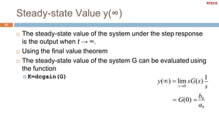
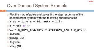
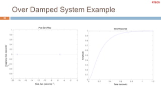
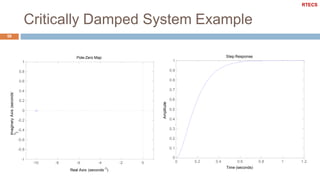
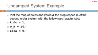
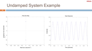
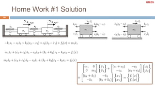
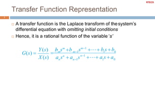
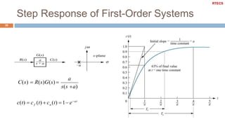
46. Under Damped System Example
47
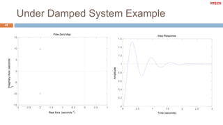
 Plot the map of poles and zeros & the step response of the
second order system with the following characteristics
 k_dc = 1; w_n = 10; zeta = 0.2;
 s = tf('s');
 G1 = k_dc*w_n^2/(s^2 + 2*zeta*w_n*s + w_n^2);
 figure
 pzmap(G1)
 axis([-3 1 -15 15])
 figure
 step(G1)
RTECS

47. Under Damped System Example
48
-3 -2.5 -2 0 0.5 1
-15
-10
-5
0
5
10
15
Pole-Zero Map
-1.5 -1 -0.5
Real Axis (seconds-1)
ImaginaryAxis(seconds-
1)
0 0.5 1 2 2.5 3
0
0.2
0.4
0.6
0.8
1
1.2
1.4
1.6
Step Response
1.5
Time (seconds)
Amplitude
RTECS

48. Under Damped System: Settling Time
49
 The settling time is the time
required for the system output to
fall within 2% percentage of the
steady state value for a step input
or equivalently to decrease to a
certain percentage of the initial
value for an impulse input.
 For a second order, underdamped
system, settling time is
approximately 3.9/(ζωn)
dn
44
Ts 



RTECS

49. Under Damped System: Percent Overshoot
50
 The percent overshoot is the
percent by which a system
exceeds its final steady-state
value.
 For a second order under
damped system, the percent
overshoot is directly related to
the damping ratio by the
following equation
100%1 2

%OS  e
RTECS

50. Under Damped System: Damping Ratio
51
 A good damping ratio is
between 0.4 and 0.8.
 Small values of  (<0.4) yield
excessive overshoot.
 Large values of  (>0.8)
responds sluggishly
RTECS

51. 52
 Step responses of second-order
underdamped systems as poles
move
 a. with constant real part
 b. with constant imaginary part
 c. with constant damping ratio
RTECS

52. Over Damped System: ζ>1
53
 If ζ>1 then the system is over damped
 Both poles are real and negative
 therefore the system is stable and does not oscillate
RTECS

53. Over Damped System Example
54
 Plot the map of poles and zeros & the step response of the
second order system with the following characteristics
 k_dc = 1; w_n = 10; zeta = 1.2;
 s = tf('s');
 G1 = k_dc*w_n^2/(s^2 + 2*zeta*w_n*s + w_n^2);
 figure
 pzmap(G1)
 figure
 step(G1)
RTECS

54. Over Damped System Example
55
-6 -4 -2 0
-1
-0.8
-0.6
-0.4
-0.2
0
0.2
0.4
0.6
0.8
1
Pole-Zero Map
-20 -18 -16 -14 -12 -10 -8
Real Axis (seconds-1)
ImaginaryAxis(seconds-
1)
0 0.2 0.4 0.8 1 1.2
0
0.1
0.2
0.3
0.4
0.5
0.6
0.7
0.8
0.9
1
Step Response
0.6
Time (seconds)
Amplitude
RTECS

55. Critically Damped System: ζ=1
56
 If ζ=1 then the system is critically damped
 Both poles are real and have the same magnitude
 Critically damped systems approach steady-state quickest without
oscillating.
RTECS

56. Critically Damped System Example
57
 Plot the map of poles and zeros & the step response of the
second order system with the following characteristics
 k_dc = 1;
 w_n = 10;
 zeta = 1;
RTECS

57. Critically Damped System Example
58
-10 -8 -2 0
-1
-0.8
-0.6
-0.4
-0.2
0
0.2
0.4
0.6
0.8
1
Pole-Zero Map
-6 -4
Real Axis (seconds-1)
ImaginaryAxis(seconds-
1)
0.2 0.4 0.8 1 1.2
0
0
0.1
0.2
0.3
0.4
0.5
0.6
0.7
0.8
0.9
1
Step Response
0.6
Time (seconds)
Amplitude
RTECS

58. Undamped System: ζ=0
59
 If ζ=0 then the system is undamped
 In this case, the poles are purely imaginary
 therefore the system is marginally stable and oscillates indefinitely.
sp   jn
RTECS

59. Undamped System Example
60
 Plot the map of poles and zeros & the step response of the
second order system with the following characteristics
 k_dc = 1;
 w_n = 10;
 zeta = 0;
RTECS

60. Undamped System Example
61
-15
-10
-5
0
5
10
15
Pole-Zero Map
ImaginaryAxis(seconds-
1)
-0.5
0
0.5
1
1.5
2
2.5
-1 -0.8 -0.6 -0.4 -0.2 0 0.2 0.4 0.6 0.8 1 0 0.5 1 1.5 2 2.5 3 3.5 4 4.5 5
Real Axis (seconds-1) Time (seconds)
Step Response
Amplitude
RTECS

61. RTECS

62. Sum-up
63
RTECS

63. References
64
 Benjamin C. Kuo and Farid Golnaraghi, “Automatic Control
Systems”, 8th edition, John Wiley & Sons,Inc.
RTECS

64. References
65
 Dingyü Xue, YangQuan Chen and YangQuan Chen, „Linear
Feedback Control, Analysis and Design with MATLAB“, 1st
edition, SIAM (Society for Industrial and Applied Mathematics),
Philadelphia
RTECS

65. Quiz
66
RTECS
• M1= 1/4 bus body mass 2500 kg
• M2= suspension mass 320 kg
• K1= spring constant of suspension system 80,000 N/m
• K2= spring constant of wheel and tire 500,000 N/m
• B1= damping constant of suspension system 350 N.s/m
• B2= damping constant of wheel and tire 15,020 N.s/m
•U= control force
Determine:
• Transfer function / Simulink models
• step response

66. Home Work #2
67
RTECS
Determine:
• select all parameters which give you suitable / accepted system behavior
• Simulink models
• step response

67. Home Work #1 Solution
68
RTECS

68. RTECS