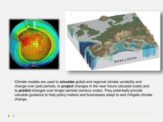
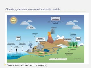
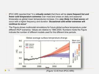
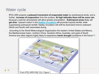
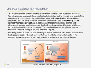
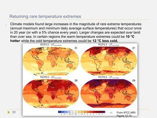
Climate models use mathematical equations and global grids to simulate and predict climate conditions based on physical principles and observational data. They show reasonable agreement with past climate trends and are used to project future climate change under different greenhouse gas emission scenarios. However, uncertainties remain regarding some processes like cloud formation. Current models estimate global warming of 0.3-1.7°C by 2100 under a low emission scenario and 2.6-4.8°C under high emissions, with greater warming over land and in polar regions. The models also predict more hot days and heat waves along with rising sea levels.

1. Climate
change
Prediction
Data collection and
presentation by
Carl Denef,
Januari 2014
1

2. Climate models
 Climate models are simplified numerical representations of the climate system constructed
with two types of essential building blocks: physical, chemical, and biological principles
founded on theory (the laws of thermodynamics and Newton’s laws of motion, for example)
and data collected from observations on climate system components. The basic models,
known as General Circulation Models (GCM), handle 3-dimentional circulation dynamics
of the atmosphere and ocean through mathematical equations.
The Earth’s surface is represented in a grid of millions of stacked cubes, with each
representing a specific area of land, ocean, sea ice, and atmosphere (see Figure next
slide). Each cube is a collection of mathematical formulas describing the processes within
that area. The mathematical equations are numerically solved by super-computers that
calculate as accurately as possible what will happen to temperatures, winds, water currents,
and many other parameters in each cube under various scenarios. For instance, models
resolve the question of what happens to temperature after a doubling of the current
atmospheric CO2 concentration. The cubes are then joined to calculate how circulation in
one cube will interact with that in surrounding grids and integrated over the globe.
Resolution of the grid cells is between 300 and 30 km. The higher the resolution the longer
the computer time needed. Even with the best supercomputers of today, calculation times
can extend over several weeks.
At present, climate projections are based on an ensemble of different models, known as
multi-model ensembles. The reason for this is that averages across different models
show better large-scale agreement with observations.
2

3.  Climate models are used to simulate global and regional climate variability and
change over past periods, to project changes in the near future (decadal scale) and
to predict changes over longer periods (century scale). They potentially provide
valuable guidance to help policy makers and businesses adapt to and mitigate climate
change.
3

4.  Reliability of climate models has to be tested against what happened with climate in the
past.[125] If a model can correctly simulate trends from a particular starting point somewhere
in the past, it can be used to predict with reasonable certainty what might happen in the
future. However, different models include different entry elements and may therefore
generate different predictions. Results can also vary due to different greenhouse gas or
aerosol inputs, the model's climate sensitivity to greenhouse gases (= the change in
temperature upon doubling of CO2 in the atmosphere), the use of differing estimates of
future greenhouse gas emissions (for example the rate of methane leakage during shale
gas extraction) and so on. A model-based prediction is therefore presented under different
scenarios with respect to humanity’s future demographic expansion and behavior. Which
scenarios are most realistic is uncertain, as the projections of future greenhouse gas and
aerosol emission are themselves uncertain.
 Certain processes represented in the model may be too complex or too small-scale to be
physically represented in the model. In that case the process is replaced by a simplified
process. This manipulation is known as parameterization. Various parameters are used in
these simplified processes. An example are clouds. Cloud formation is notoriously complex
and climate model gridboxes for clouds have a resolution of 5 km, which is much larger than
the scale of a typical cumulus cloud (1 km). Therefore the processes that such clouds
represent are parameterized.
 Because of simplification by parameterization and uncertainty in scenarios, climate models
always enclose estimates of uncertainty levels.
4

5. Climate system elements used in climate models
Source: Nature 463, 747-756 (11 February 2010)
Clouds
5

6. Reliability of climate models
 Models have accurately predicted climate change trends in the past. For example, the
vulcanic eruption of Mt. Pinatubo allowed to test the accuracy of models by entering the
eruption data and then observe how climate changed. The observed climatic response was
found consistent with the prediction. Predictions of atmospheric CO2 levels made by IPCC
in 1990 were also fully confirmed by the later observations (see slides on ‘Climate change in
the atmosphere’). Models also correctly predicted greater warming in the Arctic and over
land, greater warming at night, and stratospheric cooling.
 Other predictions underestimated climate change, such as arctic ice melting and sea
level rise predicted by the IPCC Third Assessment report. Precipitation rates also
increased significantly faster than global climate models predicted.
 Still others slightly over-estimated the rise in atmospheric methane concentrations (see
IPCC AR5 WG1).
 An important uncertainty factor in climate predictions is climate sensitivity – being the
temperature response to a doubling of the atmospheric greenhouse gas concentration –,
because it is affected by climate feedbacks. Higher climate sensitivity will result in more
warming, in case of a positive feedback.[Ref] If a negative feedback is acting, a given
greenhouse gas rise will result in less sensitivity.
 Climate models are still not well predicting the effect of clouds [Ref] , due to lack in
knowledge of cloud generation processes. Uncertainties in methane release from
permafrost and leakage during methane extraction from shale gas by fracking, are other
examples of prediction uncertainties.
6

7. Climate sensitivity
 Projections of climate change in the future are dependent on the sensitivity of the climate
system to the greenhouse radiative forcing. It is therefore essential to have an accurate
estimate of this sensitivity. Climate sensitivity is a measure of the surface temperature change
in °C per W/m2 sustained radiative forcing. In practice it is expressed as the temperature
change associated with a doubling of the concentration of CO2 in the atmosphere relative
to pre-industrial levels (~280 ppm). There are two ways to look at climate senstivity:
equilibrium climate sensitivity (ECS) and transient climate sensitivity (TCS). The former is
calculated over the time span needed to reach full equilibrium between sustained CO2
forcing and the climate system. TCS is defined as the average temperature response over a 20-
year period to CO2 doubling with CO2 increasing at 1% per year.[Ref] TCS is lower than ECS,
due to the "inertia" (slowliness) of ocean heat uptake and ice sheet feedbacks.
Doubling CO2 level results in forcing of 3.7 W/m2. In a simple physical environment a doubling
of CO2 would result in 1 °C warming. However, in the real atmosphere complex positive and
negative feedbacks are operating (water vapor, cloud and ice albedo, aerosols, ozone…),
influencing radiative forcing. The net warming effect was found to be ~3 times higher.
Feedbacks can also become stronger with time. For example ice sheets may melt at a given
time point at a much faster rate due to a sudden collapse of large ice shelves allowing massive
release of ice into the sea. Icebergs drift away to warmer water and melt, hereby decreasing
albedo, resulting in more warming. Addition of these longterm feedbacks to climate
models was found to lead to a higher value of ECS, but most climate models have not
included these feedbacks yet. Thus, future climate change may be more deleterious than
presently expected.
7

8.  Current climate models span an ECS range of 2.6–4.1 °C, most clustering around 3 °C."[Ref]
The IPCC AR5 concensus value of ECS, calculated by multimodel ensembles, is between
1.5°C and 4.5°C, is extremely unlikely <1°C, and very unlikely >6°C. Notice that
feedback contribution, being not constant over time, induces a level of uncertainty in any
climate model.
8

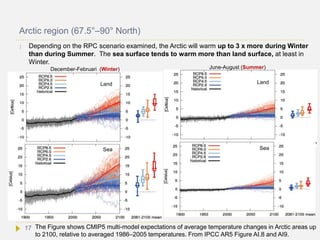
9. IPCC radiative forcing scenarios
 IPCC AR5 introduced a new set of scenarios, to project future climate change with
climate model simulations. These scenarios are called RCPs (Representative
Concentration Pathways). These are based on the radiative forcing that emission
rates would cause in the years to come. The main RCPs are RCP2.6, RCP4.5,
RCP6.0, and RCP8.5, named after the radiative forcing values that are projected
for the year 2100 i.e. +2.6, +4.5, +6.0, and +8.5 W/m2, respectively.[2]
 In the RCP8.5 scenario radiative forcing is set to reach 8.5 W/m2 by 2100 and to
continue to rise for some time thereafter. RCP6.0 and RCP4.5 are intermediate
“stabilization pathways”, where radiative forcing does not further rise after 2100. In
the RCP2.6 scenario, radiative forcing peaks at 3 W/m2 before 2050 and then declines
to 2.6 by 2100.
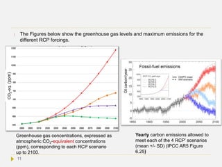
 To each forcing scenario there is a corresponding greenhouse gas level in the
atmosphere (see next slides). In order to remain within this future greenhouse gas
concentrations adopted in the RCP scenarios, the maximum cumulative fossil fuel
emissions should be not higher than 272 Gt, 780 Gt, 1062 Gt and 1687 Gt carbon
equivalents up to 2100 for RCP2.6, RCP4.5, RCP6.0, and RCP8.5, respectively (see
next slides).
9

10.  Although theoretically possible, [Ref] RCP2.6 is a
scenario difficult to attain, since 1) in 2012
radiative forcing was already 2.9 W/m2, 2) to
realize RCP2.6, atmospheric CO2 must be
stabilized at 450 ppm (see next slide) which
requires a ~70% reduction of CO2 emissions
relative to the level in 2000 (see section 5). 3)
Both RCP2.6 and 4.5 scenarios already include
‘carbon dioxide removal’ (CDR) programs (see
section 5) to remain within the radiative forcing
limit and these CDR programs are presently
considered difficult to realize on a sufficient
global scale and with sufficient safety.
 Trends in radiative forcing for 4 different
scenarios (IPCC RCP scenarios). Forcing is
relative to pre-industrial values and does not
include land use (albedo), dust, or nitrate
aerosol forcing (van Vuuren 2011).
Source
RCP8.5
RCP6.0
RCP4.5
RCP2.6
10

11.  The Figures below show the greenhouse gas levels and maximum emissions for the
different RCP forcings.
Yearly carbon emissions allowed to
meet each of the 4 RCP’ scenarios
(mean +/- SD) (IPCC AR5 Figure
6.25)
Gtcarbon/year
RCP 2.6
RCP 6.0
RCP 4.5
RCP 8.5
Greenhouse gas concentrations, expressed as
atmospheric CO2-equivalent concentrations
(ppm), corresponding to each RCP scenario
up to 2100.
CO2-eq.(ppm)
11

12. Global surface temperature predictions
 In 2001 the IPCC third assessment report (TAR) announced that, although the climate
system was so complex, scientists would never reach complete certainty about
present and future climate change, but that it is ‘much more likely than not’ that our
civilization faces severe global warming
 Since 2001, greatly improved computer models and an abundance of data have
strengthened the IPCC conclusion. The IPCC conclusions were endorsed by national
science academies of major nations and leading scientific societies.
 In 2007 the IPCC fourth assessment report (AR4) stated that “it is ‘very likely’ that
significant global warming is coming in our lifetimes. This surely brings a likelihood of
harm, widespread and grave. Depending on what will be done to restrict emissions,
we could expect the planet’s average surface temperature to rise anywhere between
about 1.4-5.8°C by the end of this century.” Notice that the lower bound is already
reached today!
 The IPCC fifth assessment report (AR5), presented in September 2013 in
Stockholm, projects a somewhat lower rise in global surface temperature in 2100.
Increase of global mean surface temperatures for 2081–2100 relative to 1986–2005 is
projected to ‘likely be’ in the range of 0.3 - 1.7°C (RCP2.6 scenario), 1.1 - 2.6°C
(RCP4.5 scenario), 1.4 - 3.1°C (RCP6.0 scenario), or 2.6 - 4.8°C (RCP8.5 scenario).
Notice that temperature during the reference period 1986–2005 had already risen by
~0.6 °C relative to the preindustrial temperature.
12

13.  IPCC AR5 reported that “it is virtually certain that there will be more frequent hot and
fewer cold temperature extremes over most land areas on daily and seasonal
timescales as global mean temperatures increase. It is very likely that heat waves will
occur with a higher frequency and duration. Occasional cold winter extremes will
continue to occur”
 The Figure shows multimodel simulations for future global surface temperature under
different RCP scenarios. Values are relative to 1985-2005. Numbers inside the Figure
indicate the number of different models used for the different time periods.
(Figure 12.40 from IPCC AR5)
Year
13

14. Land vs sea and seasonal differences
 Depending on the scenario considered, global average temperature on land surface is
anticipated to rise up to 6 °C, relative to averaged 1986–2005 temperatures, by 2100, with
little difference between Winter and Summer. Sea surface temperature will rise as well but
~2°C less.
The Figures only show land temperatures. Thin
lines denote one of 5 ensemble members per
model, thick lines the CMIP5 multi-model mean.
From IPCC AR5 Figure AI.4 and AI.5
14

15. Incidence of warm and cold days
 Warm days will drastically increase in number while cold days will decrease. The Figure
shows results from CMIP5 models under the RCP2.6, RCP4.5 and RCP8.5 scenarios.
From IPCC AR5 Figure 11.17
15

16. Regional differences
 In certain regions surface temperature anomaly for 2080-
2099 is expected to rise up to 10 °C, particulatly in the Arctic,
threatening massive melting of Greenland ice sheets. Land
surface will warm more than ocean.
 The Figure (from IPCC AR5) shows the average surface
temperature for the scenarios RCP2.6 and RCP8.5 in 2081–
2100 relative to 1986–2005, as calculated by CMIP5 multi-
models. The number of CMIP5 models used is indicated in
the upper right corner of each panel.
See NOAA animation video
h e r e, showing the projected
annual mean surface
temperature regional
distribution from 1970-2100,
(credit: NOAA Geophysical
Fluid Dynamics Laboratory).
16

17. Arctic region (67.5°–90° North)
 Depending on the RPC scenario examined, the Arctic will warm up to 3 x more during Winter
than during Summer. The sea surface tends to warm more than land surface, at least in
Winter.
Land
Sea
December-Februari (Winter)
The Figure shows CMIP5 multi-model expectations of average temperature changes in Arctic areas up
to 2100, relative to averaged 1986–2005 temperatures. From IPCC AR5 Figure AI.8 and AI9.
June-August (Summer)
Land
Sea
17

18. Antarctic region
 Temperature rise over land in Antarctica is much smaller than in the Arctic and there is little
difference between Winter and Summer.
December-Februari (Summer)
IPCC AR5 Figure A1.76 and 77
June-August (Winter)
Land Land
The Figure shows CMIP5 multi-model axpectations of average temperature changes in Arctic areas up
to 2100, relative to averaged 1986–2005 temperatures.. From IPCC AR5 Figure AI.8 and AI9.
18

19. Land ice
 IPCC AR5 concluded that it is “ ‘exceptionally unlikely’ that the ice sheets of either
Greenland or West Antarctica will suffer a near-complete disintegration during the 21st
century.” However, it may happen at a millenial time scale, because both the ocean
and the ice masses are huge, which makes it very long before heat and CO2 of the
surrounding atmosphere equilibrates. Moreover, as summarized by IPCC AR5 WG1
chapt. 13, models project that the Greenland Ice Sheet will exhibit a strongly
nonlinear and potentially irreversible response to surface warming. The mechanism
of this threshold behavior is the surface mass balance (SMB) height feedback, that is,
as the surface height is lowered due to ice loss, the higher temperature above the
near surface leads to further ice loss. This feedback is small in the 21st century but
will become important in the 22nd century. This nonlinear behaviour may be
accelerated by a reduced surface albedo caused by the continuous loss of ice sheet
extent. Models have calculated a threshold in surface warming beyond which
self-amplifying feedbacks result in a partial or near complete ice loss on
Greenland. If a temperature above this threshold is maintained over a multi-millennial
time period, the majority of the Greenland Ice Sheet will be lost on a millennial to
multi-millennial time scale. The treshhold global mean surface temperature rise to
initiate this evolution has been estimated to be 3.1 (1.9 to 4.6) °C above pre-industrial
level. Other models found this threshold at a 2.5°C rise.
Look the summarizing video
from NASA
19

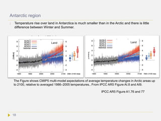
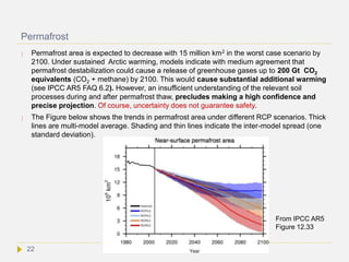
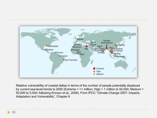
20.  Consistent with this result is that during the Middle Pliocene warm intervals, when
global mean temperature was 2°C–3.5°C higher than pre-industrial, ice-sheet models
calculated near-complete deglaciation of Greenland. Some scientists predict that
climate change may make the entire Greenland ice sheet melt in about 2,000 years.[2]
That alone would add 7m to sea level [3].
 The surface mass balance of the Antarctic Ice Sheet is projected to increase in most
models because increased snowfall outweighs melt increase. However, ice-shelf
decay due to oceanic or atmospheric warming might lead to abruptly accelerated ice
flow and loss into the sea. It remains uncertain whether East Antarctic ice sheet will
gain or loose mass [Ref]
 Also James Hansen has argued that multiple positive feedbacks could lead to
nonlinear ice sheet disintegration by increased ice flow, calving and sudden ice
shelve collapses. More surface melt water would flow to the ice sheet bed, leading to
much faster melting of the ice interior.[Ref]. Moreover, as ice sheets shed ice more and
more rapidly, in ice streams, climate simulations indicate that a point will be reached
when the high latitude ocean surface cools while low latitudes surfaces are warming.
Larger temperature contrast between low and high latitudes will drive more
powerful storms.
20

21. Arctic and Antarctic sea ice
 According to IPCC AR5 arctic sea ice will have virtually disappeared (< 1 km2 in
extent) by 2050 (37 models with RCP8.5 scenario). Antarctic sea ice extent is also
expected to decrease, altough at a considerably slower rate. Decreased sea ice extent
means less albedo and thus faster warming.
From IPCC AR5 Figure 12.28
Changes in sea ice extent as simulated by CMIP5 models over the second half of the
20th century and the whole 21st century under RCP2.6, RCP4.5, RCP6.0 and
RCP8.5 scenarios. The number of models used for each RCP is given in the legend.
21

22. Permafrost
 Permafrost area is expected to decrease with 15 million km2 in the worst case scenario by
2100. Under sustained Arctic warming, models indicate with medium agreement that
permafrost destabilization could cause a release of greenhouse gases up to 200 Gt CO2
equivalents (CO2 + methane) by 2100. This would cause substantial additional warming
(see IPCC AR5 FAQ 6.2). However, an insufficient understanding of the relevant soil
processes during and after permafrost thaw, precludes making a high confidence and
precise projection. Of course, uncertainty does not guarantee safety.
 The Figure below shows the trends in permafrost area under different RCP scenarios. Thick
lines are multi-model average. Shading and thin lines indicate the inter-model spread (one
standard deviation).
From IPCC AR5
Figure 12.33
22

23. Snow cover extent
 In all RCP scenarios Northern Hemisphere snow cover extent is anticipated to
decrease, resulting in reduced albedo and further warming. From IPCC AR5 Figure
12.32
Northern Hemisphere spring (March to April average) snow cover
extent change (in %) in the CMIP5 model ensemble, relative to the
simulated extent for the 1986–2005 reference period.23

24. Methane clathrate destabilization
 Model simulations suggest that methane from terrestrial and oceanic methane
clathrate deposits in shallow ocean regions at high latitude and in the Gulf of Mexico
are susceptible to destabilization by ocean warming. However, sea level rise will also
increase ocean mass, which enhances clathrate stability (due to higher pressure by
water). A net increase of methane release and a positive feedback on warming is
expected over multi-millennial timescales.
 A pertinent issue here is the threshold at which warming begins to mobilize seabed
methane. Reaching this threshold would initiate a “runaway” feedback warming that
characterized the PETM and EECO palaeoclimate periods. No one knows what the
threshold is. Once warming is at that treshhold, methane will enter the atmosphere
and give additional warming, which then will release more methane that then, in turn,
gives warming and so on. Runaway warming is possible and, at that stage,
uncontrollable.
24

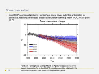
25. Sea level rise
 Sea level rise is expected to continue for
centuries, even millenia, even when
anthropogenic carbon emissions would
stabilize at the present level[13] This is
because the sea level contribution from ice
sheets continues over these time scales. In
2007, the IPCC AR4 projected that during the
21st century, sea level will rise another 18 to
59 cm, but these numbers do not include
"uncertainties in climate-carbon cycle
feedbacks nor do they include the full effects
of changes in ice sheet flow".[Ref] As shown in
the Figure, IPCC AR5 predicts similar sea
level rise. Projections assessed by the US
National Research Council[Ref] suggest
possible sea level rise over the 21st century
of between 56 cm and 2 m.
The predicted upper limit of sea level rise remains highly uncertain, due to the incomplete
understanding of fast ice streams and glacier collapse that are major contributors of ice
delivery to the sea and sea level rise (See Nature 461, 971-975, 2009).
25

26. Ultimate sea level rise
 In a recent article in PNAS (July 15, 2013), a combination of
palaeoclimate data with simulations by models was used to
estimate the future sea-level commitment on a
multimillennial time scale. It was found that oceanic
thermal expansion and the Antarctic Ice Sheet will contribute
quasi-linearly, with 0.4 m/°C and 1.2 m/°C of warming,
respectively. The contribution from glaciers saturates earlier
while the response of the Greenland Ice Sheet is
nonlinear. As a consequence sea-level rise is committed to
approximately 2.3 m/°C within the next 2,000 years. Since a
rise in temperature of at least 4 °C, relative to 1990, is
expected by 2100 under a worst case scenario, at least a 10
m rise in global sea level is expected within 2 millennia
even when no further rise in temperature would occur.
ocean warming
mountain glaciers
Greenland ice sheet
Antarctic ice sheet
total sea level
The Figure shows modelled Sea level rise contributions over
the next 2000 years from: ocean warming (a), mountain
glaciers (b), Greenland (c) and Antarctic (d) ice sheets, plotted
against temperature rise from 1 to 4 °C. The total sea level rise
(e) is about 2.3m per °C of warming above pre-industrial.
26

27.  The PNAS paper also calculated the
regional differences of sea level rise
under a 1, 2, 3 and 4 °C sustained
temperature rise (see Figure). Even
under the « safe » 2 °C temperature
rise, many regions in the World will see
a 5-6 m sea level rise
 The theoretical maximal sea level rise
would be reached if all land ice would
melt. According to IPCC AR4 this is 7
m if Greenland ice melts and 57 m if
Antarctic Ice Sheets melt. Greenland
melting alone would inundate most
coastal cities over the world. The
total possible contribution of glaciers
(i.e., all of the land ice excluding the ice
sheets) is limited to ∼0.5-0.6 m (From
IPCC AR5, Ch. 4 and ref 22 in PNAS).
27

28. Ocean acidification
 The average pH of ocean surface waters today has
fallen by about 0.1 unit (from about 8.2 to 8.1) since
1765 and will further fall to 7.7 by the end of this
century under the RCP8.5 scenario. To illustrate the
potential damage to life and ecosystems, look at what
happens to human cells during acidosis. The normal
pH in human blood ranges between 7.35 and 7.45.
Irreversible cell damage occurs when pH falls below
6.8 or rises above 7.8. However, it remains uncertain
how much and how fast pH could change to allow
ecosystems in the ocean to adapt.
 Notice that under normal seawater conditions, the
hydrogen ions that are produced from CO2 dissolved in
water will combine with carbonate ion (CO3
2– ) to
produce HCO3
–. Doubling of CO2 levels in the
atmosphere relative to preindustial levels would
reduce carbonate ion concentration from 228 to 144
µmol/kg (IPCC AR5 FAQ 3.2, Table 1). Thus, uptake of
anthropogenic CO2 into the oceans consumes
carbonate ions, lowering availability of the building
blocks of skeletons and shells in marine organisms.

From IPCC AR5 Figure 6.28
28

29. Ocean oxygen content
 About three O2 molecules are lost every time a single CO2 molecule is produced by fossil
fuel combustion. A 0.0317% decline in atmospheric oxygen has been recorded thus far (for
the period 1990 to 2008) and is expected to drop further, as a consequence of the warming-
induced decline in dissolved oxygen in the ocean upper 500 m. A second cause is the
slowing down of the thermohaline circulation, resulting in less oxygen carried from the
surface layers of the water into the deeper layers. Oxygen is the most important limiting
factor on the growth of many marine organisms. Lowering oxygen makes it more difficult for
these animals to find food, avoid predators, and reproduce.
From IPCC AR5 Figure 6.30
Simulated changes in dissolved O2 (mean and model
range as shading) relative to 1990s for
RCP2.6,RCP4.5, RCP6.0 and RCP8.5.
Multi-model simulated changes in dissolved O2
(mmol/m3) for 2090-2100 period relative to the
1990s for RCP8.5
29

30. Thermohaline circulation
 Thermohaline circulation is a major driver of climate. As reported by IPCC AR5, it is
very likely that the thermohaline circulation will weaken over the 21st century relative
to preindustrial values. Weakening could occur as a consequence of high freshwater
runoff from rapidly melting Greenland ice sheet. The weakening in 2100 is projected to
be about 20–30% for the RCP4.5 scenario and 36–44% for the RCP8.5 scenario. The
consequence will be cooling of the Atlantic Northern Hemisphere, as weakening of the
thermohaline circulation diminishes the influx of warm tropical water into the northern
Atlantic Ocean. Western Europe would then experience cold winters.
30

31. Water cycle
 IPCC AR5 projects a poleward movement of evaporated water by extratropical winds, and a
further increase of evaporation from the surface. At high latitudes there will be more rain,
because a warmer atmosphere will allow greater precipitation. Subtropical areas likely will
get drier. Upward motion in the Hadley circulation will promote tropical rainfall, while
suppressing subtropical rainfall. Hadley circulation will shift its downward branch poleward
(North and South) with associated drying.
 According to the World Meteorological Organization the western United States and Mexico,
the Mediterranean basin, northern China, Southern Africa, Australia, and parts of South
America are other regions highly likely to experience harsh drought conditions in the future (9).
From IPCC AR5 FAQ 12.2, Figure 1
31

32. 
32
Look at the video animation of global rainfall by NASA-
Goddard Space Flight Center Scientific Visualization Studio
The video shows the frequency
that regions receive no rain
(brown), moderate rain (tan), and
very heavy rain (blue). The
occurrence of no rain and
heavy rain will increase, while
moderate rainfall will decrease.

33. Global and regional precipitation change
 Multimodel projections show a positive trend in global precipitation (from October to March)
over land and over sea, but it is relatively small even under the worst case scenario
RCP8.5. Higher latitude and tropical regions will experience the highest precipitation
increases. Subtropical zones will be drier.
Land (Oct-March)
Sea (Oct-March)
From IPCC AR5 Figure AI.6; From IPCC AR5 Figure 12.22
33

34. Wettest days incidence
 Extreme precipitation events will become more pronounced.
From IPCC AR5 Figure 11.17 From IPCC AR5 Figure 12.26
34

35. Monsoon circulation and precipitation
 The major monsoon systems are the West African and the Asian-Australian monsoons.
Warming-related changes in large-scale circulation influence the strength and extent of the
overall monsoon circulation. Several studies show an intensification of the rainfall
associated with the Indian summer monsoon, concomitant with a weakening of the
summer monsoon circulation. In addition, anthropogenic land use change and
atmospheric aerosol loading can lower the land-sea temperature difference and hence
further weaken the monsoon circulation. The net effect is more precipitation, due to
enhanced moisture transport into the monsoon regions.
 For many people in India it is the variability of rainfall on shorter time scales that will have
the biggest impacts. Intense heavy rainfall may lead to flooding while breaks in the
monsoon of a week or more, may lead to water shortage and agricultural drought.
From IPCC AR5 FAQ 14.2, Figure 135

36. Extreme weather events
From IPCC ‘Special Report on
Managing the Risks of Extreme
Events and Disasters (SREX)’.36

37. Temperature extremes
 It is virtually certain
that there will be more
hot and fewer cold
extremes by the end of
this century. The
temperature of the
coldest day of the year
will undergo larger
increases than the
warmest day (up to 7
°C and in many
regions up to 11 °C),
paricularly in the
northern hemisphere
at higher latitudes.
Multi-model projections of changes in the annual minimum of the minimum daily temperature and
annual maximum of maximum daily temperature, (relative to a 1981–2000 reference period) under
the RCP8.5 scenario. IPCC AR5 Figure 12.13
37

38.  There will be up to 7-25
frost days (below 0°C)
less by 2100,
depending on the
scenario considered.
On the other hand, the
number of tropical
nights (above 20°C)
will go up with 60 in the
worst case scenario.
The fall in frost days will
be more pronounced at
higher latitudes in the
Northen Hemisphere,
while tropical nights will
increase most at
tropical and subtropical
latitudes (in some areas
up to 90 days).
There will be more record high than record cold temperatures. Meehl et al. (2009) calculated that
the current ratio of 2 to 1 for record daily maxima to record daily minima temperatures in the United
States will become approximately 20 to 1 by the mid 21st century and 50 to 1 by late century.
IPCC AR5 Figure 12.13
38

39. Returning rare temperature extremes
 Climate models found large increases in the magnitude of rare extreme temperatures
(annual maximum and minimum daily average surface temperatures) that occur once
in 20 year (or with a 5% chance every year). Larger changes are expected over land
than over sea. In certain regions the warm temperature extremes could be 10 °C
hotter while the cold temperature extremes could be 12 °C less cold.
From IPCC AR5
Figure 12.14
39

40. Humid heat waves
 Human discomfort, morbidity and mortality during heat waves depend not only on temperature
but also specific humidity. Coastal regions display abundant atmospheric moisture and
therefore are expected to experience the greatest heat stress changes.In mediteranian areas the
number of combined tropical nights and hot days per year will drastically increase.
From European Environment Agency
40

41. Droughts
 Consecutive dry days will increase in number, particularly in North and South Africa,
South America, Southern Europe and Australia.
 While previous long-term droughts in Southwest North America arose from natural
causes, climate models project that this region will undergo progressive aridification as
part of a general drying and poleward expansion of the subtropical dry zones
caused by global warming.
Data are multimodel average
changes in the period 2081-
2100 relative to the 1981–
2000 reference period. From
IPCC AR5 Figure 12.26
41

42.  Droughts with an intensity that only occurred once in 100 year, will be up to 10 times
more frequent in some regions in southern Europe.
42

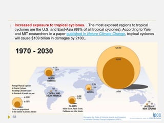
43. Tropical cyclones
 The intensity of Atlantic hurricanes is expected to increase as the ocean warms. More
heat means more energy to drive atmospheric circulations, evaporation and ocean-air
interactions. Although there have been dramatic improvements in predicting the
trajectory of tropical cyclones, the largest uncertainty exists in the prediction of tropical
cyclone intensity. The frequency of category 4 and 5 tropical cyclones over the 21st
century is expected to increase, the largest increase projected to occur in the Western
Atlantic, North of 20 degrees[Science 327, 454–458 (2010)]. A doubling of atmospheric CO2 may
increase the frequency of the most intense cyclones [J. Clim. 17, 3477 (2004)].
 On the other hand, there is evidence that the strong cyclones cause a large amount
of ocean mixingRef, pumping heat from the surface down into the oceanic interior,
which is then redistributed over the globe, particularly through upwelling of the heat in
the equatorial Eastern Pacific, where El Niño originates. This may turn the globe into a
permanent El Niño condition[Ref], which will favor global warming in a closed positive
feedback loop.
 In combination with sea level rise and tides, storm surges may cause more floods.
 Moreover, climate simulations indicate that, as ice sheets release ice more and more
rapidly in ice streams and hence cool the ocean at high latitude, a point will be
reached when the high latitude ocean surface cools while low latitudes surfaces are
warming. Larger temperature contrast between low and high latitudes will induce
more powerful storms.[Ref]
43

44. Millenial scale projections of global warming and
CO2 residence time
 It is very likely that large fractions of emitted CO2 will remain in the
atmosphere for at least 1000 years after anthropogenic emissions have
stopped. Temperature will remain elevated for an even longer time due to
the very slow mixing of heat with the deep ocean waters and the slow transfer of
already stored heat in the oceans back into the atmosphere. This extremely long
inertia times makes climate change irreversible on time scales relevant to
human life (see next slide and IPCC AR5 Box 6.1).
 There is high agreement between models that ocean warming and circulation
changes will reduce the rate of CO2 uptake in the Southern Ocean and
North Atlantic, which will amplify warming.
44

45.  This Figure shows model-
simulated millenial evolution,
under the 4 RCP scenarios, of
atmospheric CO2 levels and global
mean surface temperature after
CO2 emissions up to 2300,
followed by zero emissions
after 2300,.
45
ppm
From IPCC AR5 Figure 12.44
adapted.
The drop in temperature in 2300 is a
result of eliminating all CO2
emissions. Shadings and bars
denote the minimum to maximum
range. The dashed line on panel (b)
indicates the pre-industrial CO2
concentration.

46.  This Figure shows model-simulated
changes of global mean surface
temperature and atmospheric CO2
levels up to the year 3000, under the 4
RCP forcing scenarios, up to 2300
followed by a constant (year 2300
level) radiative forcing (Zickfeld et
al., 2013). Under RCP8.5, radiation
will reach 12.5 W/m2 by 2300. Notice
that CO2 will rise to 7 x preindustrial,
and average temperature will be 8 °C
higher. Shadings and bars denote the
minimum to maximum range. The
dashed line on panel (a) indicates the
pre-industrial CO2 concentration.
 Other models predict a temperature
increase above 8 °C by 2300 (see
IPCC AR5 Figure 12.40).
From IPCC AR5 Figure 12.43
46

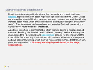
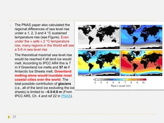
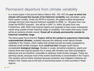
47. Is the World inhabitable with a 10 °C rise in
average global temperature?
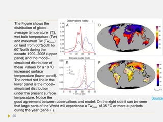
 The human body at rest cannot survive in an ambient sustained wet bulb temperature
(Tw) ≥35°C. The highest Tw (Twmax) anywhere on Earth today is ~30 °C and the most-
common Twmax is 26–27 °C.[Ref] About 58% of the world’s population in 2005 resided in
regions where Twmax ≥ 26 °C. A recent climate model simulation study reported that a
global average temperature rise of 5 °C would result in a Twmax > 35 °C in some
locations. [Ref] For an 8.5 °C increase the most-common value of Twmax would be 35 °C
, which is incompatible with human life. With a 10 °C rise, many regions would
experience a Tw = 35 °C at a particular time each year, even in Siberia (see next
slide). It looks therefore that most of the World would be practically inhabitable
in a 10 °C warmer climate. At this temperature grain and agricultural production
would suffer very much or be destroyed, causing a food crisis. Humans could air-
condition their houses but deployment this over the World will be economically and
energetically extremely demanding and a power failure would be life threatening.
People working outside cannot work in air-conditioned environments and these would
rapidly develop hyperthermia. Poorer countries, which are located in tropical and
subtropical regions, will be hit the most.
 During the PETM and EECO average global surface temperature rose 7-14 °C, which
is comparable to the study mentioned above. The question is then: How life could
have adapted to that hothouse? Humans have a body temperature of 37 °C but
many other mammals have a 2 °C and birds a 5 °C warmer body temperature[Ref] [Ref].
47

48. Non-human mammals and birds therefore may be more heat-tolerant than humans.
Just before the onset of the PETM mammals were small-sized (average = 1 kg)[Ref] [Ref]
[Ref]). This may have allowed their survival at that time, as small body mass is better
adapted to high temperatures (higher surface/mass ratio allowing better cooling).
Bioevolution during the PETM occurred over a time span of 20,000 years. In contrast,
anthropogenic warming extends over a few centuries, too short for a significant
evolutionary adaptation in heat tolerance.
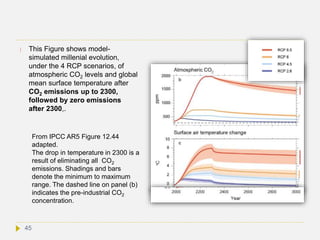
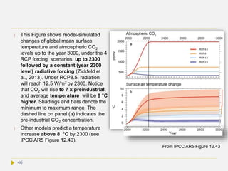
 But is this a realistic scenario? RCP8.5 is considered by IPCC as a worst case
scenario maintained up to 2300. If this scenario becomes reality, humans will have
made the World ~5-10 °C warmer by then. Atmospheric concentration would have
risen to ~7 x preindustrial. If fossil fuel burning would further increase, we would be
on the way to a 10 °C rise. However, it looks highly unlikely that humans would not
reduce greenhouse gas emissions as soon as the impacts of climate change become
frightening, which is definitely earlier than 2300. Nonetheless, the temperatures
reached at that time would decrease only very slowly, even under strong reductions or
complete elimination of CO2 emissions. Temperature might even increase temporarily
due to an abrupt reduction of short-lived aerosol emissions and, hence, of aerosol
negative forcing – see IPCC AR5 Ch. 12). Heat stored in the ocean will be released at
an even slower rate. Thus, we would be forced to live in a World with climate
disasters in many regions for many centuries.
48

49.  Can a 10 °C rise be reached if we burn all fossil energy? Since it takes
more than 1000 years for emitted CO2 to be removed, the cumulative amount of
emitted CO2 determines future climate. The amount of fossil fuels still available
ranges between 7,300-15,000 gigatonnes carbon equivalent. James Hansen
calculated[Ref] that burning this amount would increase Earth’s average surface
temperature with 16°C. It would make the World practically inhabitable.
49

50. Source
The Figure shows the
distribution of global
average temperature (T),
wet-bulb temperature (Tw)
and maximum Tw (Twmax)
on land from 60°South to
60°North during the
decade 1999–2008 (upper
panel) and the model-
simulated distribution of
these values for a 10 °C
increased surface
temperature (lower panel).
The dotted red line in the
lower panel is the model-
simulated distribution
under the present surface
temperature. Notice the
Observations today
50
good agreement between observations and model. On the right side it can be seen
that large parts of the World will experience a Twmax of 35 °C or more at periods
during the year (panel F).

51. Permanent departure from climate variability
 In a recent paper in the journal Nature (Nature 502, 183–187) the year at which the
climate will exceed the bounds of its historical variability was calculated, using
Earth system models. Under the RCP4.5 scenario, the global surface temperature
average will have risen beyond historical variability by 2069, i.e. 56 years from now.
Under the RCP8.5 scenario, this will be in 2047 i.e. within 34 years from now.
Furthermore, after 2050 most tropical regions are expected to have every subsequent
month lying outside of their historical range of variability. This means that every month
will be an extreme climatic record. Ocean pH is already permanently outside its
historical variability range.
The same paper found that the Tropics will be the earliest to experience historically
unprecedented climates, probably because the relatively small natural climate
variability in the Tropics, which makes that climate bounds are easily surpassed by
relatively small climate changes. Such small but fast changes could induce
considerable biological damage. Studies in corals, terrestrial ectoderms, plants and
insects show that tropical species live in areas with climates near their physiological
tolerances and are therefore vulnerable to relatively small climate changes. These are
alarming results, because most of the world’s biodiversity is concentrated in the Tropics.
The situation will be further impaired because protection and mitigation initiatives are
limited in the Tropics due to the lack of economical power of most countries in these
regions.
51

52.  These findings have enormous consequences on human society because under
RCP4.5 conditions roughly 1 billion people will live in areas where climate will
exceed historical bounds of variability by 2050 and these people have no historical
responsibility for the climate changes. Under RCP8.5 conditions this will be 5 billion
people.
52

53. Ecosystems[Ref]
 In terrestrial ecosystems, the earlier timing of spring events, and poleward and upward
shifts in plant and animal range, have been linked with high confidence to recent
warming. Future climate change is expected to particularly affect certain ecosystems,
including tundra, mangroves, and coral reefs. It is expected that most ecosystems will
be affected by higher atmospheric CO2 levels, combined with higher global
temperatures. Overall, it is expected that climate change will result in the extinction of
many species and reduce ecosystems diversity. Since ecosystems provide many
goods and services to humans and other living systems in a mutually dependent
manner, the consequences of ecosystem losses may become a very serious problem.
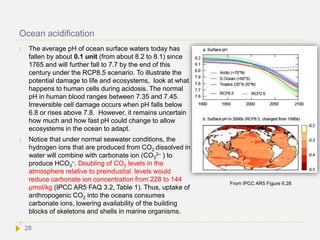
 The current rate of ocean acidification is many times faster than at least the past 300
million years, which included four mass extinctions that involved rising ocean acidity,
such as the Permian mass extinction, which killed 95% of marine species. By the end
of the century, acidity changes would match that of the Palaeocene-Eocene Thermal
Maximum (see slides on palaeoclimate), which occurred over 5000 years and killed
35–50% of benthic foraminifera[Ref] . It has been shown that corals, coccolithophore
algae, coralline algae, foraminifera, shellfish and pteropods experience reduced
calcification when exposed to elevated CO2 in the oceans. [Ref]
 Warming of the surface ocean, combined with ocean acidification and reduction
in ocean oxygen concentration will have potentially nonlinear multiplicative impacts
on biodiversity and ecosystems and each may increase the vulnerability of ocean
53

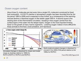
54. systems, triggering an extreme impact. In the upper 500 m of the oceans oxygen
levels range between 50 and 300 mmol/m3, with levels highest at higher latitudes.
[Ref] Many marine organisms cannot survive under hypoxic conditions (oxygen
between 60 to 120 mmol/m3 depending on the species).[Ref] [Ref] Multiple studies
reported an impressive increase in the number of hypoxic ocean zones and their
extension, severity, and duration.[Ref] There are several examples in palaeoclimate
records that extreme ocean hypoxia led to the loss of 90% of marine animal taxa.[Ref]
The slowing down of the ocean’s circulation also results in fewer nutrients from the
deep layers into the ocean surface, which endangers oxygen-producing phytoplankton
that live in the ocean surface. Phytoplankton organisms produce half of the
world’s oxygen output (the other half is produced by plants on land). Hence, with
decreasing numbers of these oxygen producers, the level of oxygen in the ocean is
bound to decline further, entailing dramatic shortages in food supply.
As reported by the IPCC AR5 WG1 chapt. 12, models consistently predict an increase
in dry season length, and a 70% reduction in the areal extent of the rainforest by
the end of the 21st century under a worst case scenario. If the dry season becomes
too long, wildfires combined with human-caused fire ignition, can undermine the
forest’s resiliency. Fire and deforestation could act as a trigger to abruptly and
irreversibly change the forest ecosystem. Forests purify our air, improve water
quality, keep soils intact, provide us with food, wood products and medicines, protect
54

55. against heat, and are home to many of the world’s most endangered species. An
estimated 1.6 billion people worldwide rely on forests for their livelihoods, including 60
million indigenous people who depend on forests for their subsistence. Forests also
help protect the Planet from climate change by absorbing massive amounts of CO2.
Boreal forests could tip into a different vegetation state under climate warming. It
should be noted, however, that uncertainties on the likelihood of it are very high, due
to large gaps in knowledge of the ecosystemic and plant physiological
responses to warming (see IPCC AR5 WG1 chapt. 12).
55
Look at a movie on plant
productivity decrease
despite more CO2 availability

56. Socio-economic consequences
 Water and food supply:
Ocean warming, oxygen depletion, and acidification will result in reduction in primary
productivity of living species and, hence, in ocean goods and services for humans.
More floods will destroy more crops. Less water means less agriculture, food and
income. Crop yield will be decreased in drier areas.
The Himalayan glaciers provide water for drinking, irrigation, and other uses for about
1.5 billion people. Since most glaciers in the Hindu Kush Himalayan region are
retreating, the concern has been raised that over time the region's water supply may
be threatened. However, recent studies show that at lower elevations, glacial retreat is
unlikely to cause significant changes in water availability over the next several
decades. Other factors, such as groundwater depletion and increasing water use by
human activity could have a greater impact than the decrease of glacier water. On the
other hand, higher elevation areas could experience less water flow in some rivers if
current rates of glacier retreat continue, but shifts in rain and snow due to climate
change will likely have a greater impact on regional water supplies[Ref] . Whatever the
reason, climate change may likely threaten water supply and consequently food
supply.
Glacier recession reduces the buffering role of glaciers, hence inducing more floods
during the rainy season and more water shortages during the dry season.
56

57.  Human health:
Climate change caused >100,000 deaths/year at present. By 2030, climate change is
estimated to indirectly cause nearly one million deaths a year and inflict 157 billion
dollars in damage in terms of today's economy. Read more here
Diseases that are caused by prolonged exposure to heat include cramps, fainting, and
heatstroke, and these can eventually lead to death. The key to preventing such health
hazards is the accessibility of air conditioning. But as heat extremes will become
more common, the reliance on air conditioning could cause problems for people in
areas that are both adapted to high temperatures and those that are not. In regions
like the southern United States, which are today accustomed to heat and where air
conditioning is common, the increasing demands on power generators could become
problematic if heat waves increase. In the Northwestern United States and Europe,
where few places have air conditioning today, problems include making air
conditioning available and ensuring that there is enough power to supply them.
An important inherent factor deteriorating human health is that emissions inherently
cause pollution and pollutants caused 400,000 premature deaths in Europe alone.
57

58.  Increased exposure to tropical cyclones. The most exposed regions to tropical
cyclones are the U.S. and East-Asia (88% of all tropical cyclones). According to Yale
and MIT researchers in a paper published in Nature Climate Change, tropical cyclones
will cause $109 billion in damages by 2100,.
58

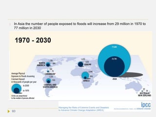
59.  Increased exposure to floods.
An increase in the frequency or intensity of floods would be catastrophic in many low-
lying places around the World. Asian countries are particularly at risk, as low-lying
areas (like river deltas and small islands) are densely populated. In Bangladesh
alone, over 17 million people live at an elevation of less than 1 m above sea level, and
millions more inhabit the flat banks of the Ganges and Brahmaputra Rivers. Another
consideration is that poorer countries like Bangladesh do not have the financial
resources to relocate their citizens to lower risk areas, nor are they able to create
protective barriers. Read more
The Organization for Economic Co-Operation and Development announced the 10
cities most vulnerable to flooding. Six are in Asia: Mumbai, Shanghai, Ho Chi Minh
City, Calcutta, Osaka, and Guangzhou. The other four are in the United States: New
York City, Miami, Alexandria, and New Orleans. All are coastal, low-lying, and
densely populated[12].
Floodwaters can contaminate drinking water, and sea level rise can lead to the
contamination of private wells, with local catastrophic results.
59

60.  In Asia the number of people exposed to floods will increase from 29 million in 1970 to
77 million in 2030
60

61.  Hotspots for vulnerability
River Deltas and megadeltas are highly vulnerable to the impacts of climate change,
particularly sea-level rise and changes in river runoff. Many of them also experience
strong urban area expansion, collecting more and more people in small land spots.
A global sample of 40 deltas inhabited by ~300 million people was studied for the
impact of climate change. This analysis showed that much of the population of these
40 deltas is at risk through coastal erosion and land loss, primarily as a result of
decreased sediment delivery by the rivers (due to the effects of water use and
diversion, and declining sediment input as a consequence of water entrapment in
dams). This phenomenon of land subsidence augments relative sea-level rise.
Many people are already subject to flooding from both storm surges and seasonal
river floods.
61

62. 62
Relative vulnerability of coastal deltas in terms of the number of people potentially displaced
by current sea-level trends to 2050 (Extreme = >1 million; High = 1 million to 50,000; Medium =
50,000 to 5,000; following Ericson et al., 2006). From IPCC “Climate Change 2007: Impacts,
Adaptation and Vulnerability”, Chapter 6

63.  Transport infrastructure
 Transport infrastructure is vulnerable to extremes in temperature, floods from
precipitation and rivers, and storm surges.
 Since 80 % of global trade in goods is transported by sea, freight-handling ports
and their road and rail connections, will be at high risk for serious damage from
storm surges and floods, particularly in regions with very low elevation above sea
level such as the U.S. Gulf Coast.
63

64. Heat waves can cause road pavement to soften and expand and can place stress on
bridge joints. Heat waves or floods can also limit construction activities, particularly in
areas with high humidity. With these changes, it could become more costly to build
and maintain roads and highways.
Storms and floods may
damage oil pipe lines and
cause oil spills.
64

65.  Impacts on tourism (from IPCC, Managing the Risks of Extreme Events and
Disasters to Advance Climate Change Adaptation) (SREX).
These include:
 Direct impacts on tourist infrastructure (hotels, access roads, etc.), on operating
costs (heating/cooling, snowmaking, irrigation, food and water supply, evacuation,
and insurance costs), on emergency preparedness requirements, and on business
disruption (e.g., sun-and-sea or winter sports holidays)
 Indirect environmental change impacts of extreme events on biodiversity and
landscape (e.g. coastal erosion), which may negatively affect the quality and
attractiveness of tourism destinations
 Adverse weather conditions or the occurrence of an extreme event can reduce a
touristic region’s popularity during the following season.
65

66.  Environmental refugees:
There are currently between 25-30 million refugees worldwide as a consequence of
climate events, and their numbers are expected to rise to 200 million by
2100.[14]Unlike traditional refugees, environmental refugees are not recognized by the
Geneva Convention or the United Nations High Commission on Refugees (UNHCR),
and therefore do not have the same legal status in the international community. Most
threatened are people in developing countries - in particular, people in low-lying
regions, on small islands, and arid regions that suffer from drought across North
Africa, farm regions dependent on river water from glacier and snow melt, and regions
of Southeast Asia facing changes in monsoon patterns. These countries have the
least economical power to adapt to climate change.
Most international statements on human rights in relation to climate change have
emphasized the potential adverse impacts of climate change on the human rights to
life, health, food, water, housing, development, and self-determination.[13] These rights
are enumerated in the UN conventions of international human rights law, though not
all UN members or UNFCCC parties have signed these conventions.
66

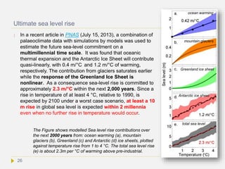
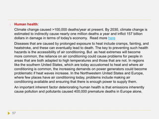
67.  Worsening of human conflicts.
The impact of climate change will make
the poorest communities across the
world poorer. Many of them experience
conflict and instability, on top of poverty,
which exposes them to a dual risk. The
impact of climate change may entail
more violent conflict, which in turn
counteracts governments and people to
adapt to climate change. Thus, climate
change and violent conflict create a
potential vicious circle of destruction, if
not properly cared of by the international
community.
 International peacebuilding NGO
International Alert named 46 countries
where climate change effects may
interact with economic, social, and
political forces to create a high risk of
violent conflict.[15]
1. Afghanistan
2. Algeria
3. Angola
4. Bangladesh
5. Bolivia
6. Bosnia & Herzegovina
7. Burma
8. Burundi
9. Central African Republic
10. Chad
11. Colombia
12. Congo
13. Côte d’Ivoire
14. Dem. Rep. Congo
15. Djibouti
16. Eritrea
17. Ethiopia
18. Ghana
19. Guinea
20. Guinea Bissau
21. Haiti
22. India
23. Indonesia
24. Iran
25. Iraq
26. Israel & Occupied
Territories
27. Jordan
28. Lebanon
29. Liberia
30. Nepal
31. Nigeria
32. Pakistan
33. Peru
34. Philippines
35. Rwanda
36. Senegal
37. Sierra Leone
38. Solomon Islands
39. Somalia
40. Somaliland
41. Sri Lanka
42. Sudan
43. Syria
44. Uganda
45. Uzbekistan
46. Zimbabwe
67

68. Combined climate change impacts (Europe)
The Figure shows predictions (using CCLM models under an IPCC scenario between
RCP6.0 and RCP8.5) of climate change impacts for the period 2070-2100, based on
regional sensitivity and exposure to climate factors and with a weighted combination of
physical, environmental, social, economical and cultural impact parameters. From
IRPUD Espon Climate Project, 2011 ©
68

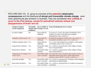
69. Potentially abrupt and irreversible changes
(”tipping points”)
 According to IPCC AR5 WG1 Chapter 12, abrupt climate change is defined as a
large-scale change in the climate system that develops over a few decades or less,
persists for at least a few decades, and causes substantial disruptions in human and
natural systems. Abrupt changes arise from nonlinearities within the climate system.
They are therefore inherently difficult to assess and their timing is difficult to predict.
Nevertheless, progress is being made on the basis of early warning signs for abrupt
climate change.
 AR5 defines a perturbed climate state as irreversible (also known as a “tipping
point”), if the timescale of recovery from this state via natural processes is
significantly longer than the time it took for the climate system to reach this perturbed
state. According to this definition climate change resulting from CO2 emissions are
irreversible, due to the long residence time of the CO2 in the atmosphere and the
inertia of oceans to store the CO2 and the resulting warming (see next slides). A
tipping point is a point such that no additional forcing is required for large change and
impacts to occur.[8] If climate change reaches a state that causes serious disconfort to
humans, potential catastrophic situations emerge for centuties, and even millenia.
69

70.  IPCC AR5 WG1 Ch. 12 gives an overview of the potential catastrophic
consequences and the likelihood of abrupt and irreversible climate change, even
when greenhouse gas emission is reversed. They are considered very unlikely to
occur in the 21st century, except for permafrost methane release and
disappearance of Arctic sea ice.
70

71. When will the next Ice Age begin?
 Changes in future solar radiation by variations in the Earth’s orbit around the sun
(orbital forcing) can be accurately calculated, since the periods of the Milankovitch
cycles are precisely known (see ‘Key concepts’). This allows to predict the onset of
the next glacial period. Since the glaciation threshold depends also on the
atmospheric CO2 concentration, several different models have been run to investigate
the response to orbital forcing in the future for different atmospheric CO2 scenarios.
The results consistently show that a new glacial period will not develop within the
next 50,000 years, if atmospheric CO2 concentration remains above 300 ppm.
71

72. 
72