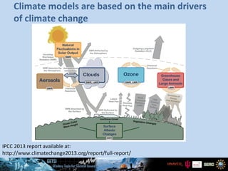
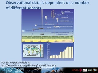
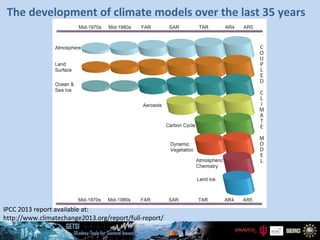
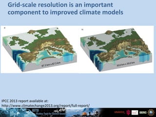
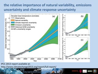
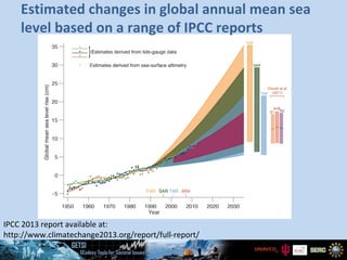
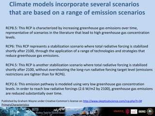
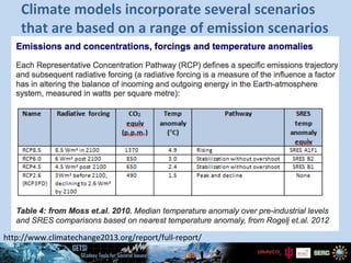
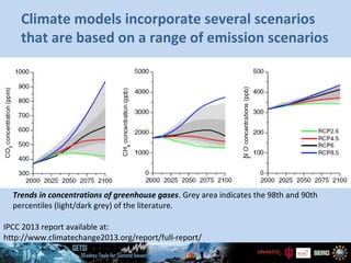
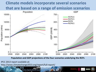
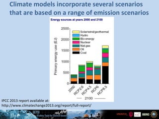
IPCC 2013 report available at:
http://www.climatechange2013.org/report/full-report/
Climate models are based on the main drivers
of climate change
IPCC 2013 report available at:
http://www.climatechange2013.org/report/full-report/
Observational data is dependent on a number
of different sensors
The development of climate models over the last 35 years
IPCC 2013 report available at:
http://www.climatechange2013.org/report/full-report/
Grid-scale resolution is an important
component to improved climate models
IPCC 2013 report available at:
http://www.climatechange2013.org/report/full-report/
the relative importance of natural variability, emissions
uncertainty and climate response uncertainty
IPCC 2013 report available at:
http://www.climatechange2013.org/report/full-report/
Estimated changes in global annual mean sea
level based on a range of IPCC reports
IPCC 2013 report available at:
http://www.climatechange2013.org/report/full-report/
RCP8.5: This RCP is characterized by increasing greenhouse gas emissions over time,
representative of scenarios in the literature that lead to high greenhouse gas concentration
levels.
RCP6: This RCP represents a stabilization scenario where total radiative forcing is stabilized
shortly after 2100, through the application of a range of technologies and strategies that
reduce greenhouse gas emissions.
RCP4.5: This RCP is another stabilization scenario where total radiative forcing is stabilized
shortly after 2100, without overshooting the long-run radiative forcing target level (emissions
restrictions are tighter than for RCP6).
RCP2.6: This emission pathway is modeled using very low greenhouse gas concentration
levels. In order to reach low radiative forcings (2.6 W/m2 by 2100), greenhouse gas emissions
are reduced substantially over time.
Published by Graham Wayne under Creative Common’s license on http://www.skepticalscience.com/rcp.php?t=3#
PrimaryCharacteristics
Climate models incorporate several scenarios
that are based on a range of emission scenarios
Climate models incorporate several scenarios
that are based on a range of emission scenarios
http://www.climatechange2013.org/report/full-report/
Trends in concentrations of greenhouse gases. Grey area indicates the 98th and 90th
percentiles (light/dark grey) of the literature.
Climate models incorporate several scenarios
that are based on a range of emission scenarios
IPCC 2013 report available at:
http://www.climatechange2013.org/report/full-report/
Population and GDP projections of the four scenarios underlying the RCPs
Climate models incorporate several scenarios
that are based on a range of emission scenarios
IPCC 2013 report available at:
http://www.climatechange2013.org/report/full-report/
IPCC 2013 report available at:
http://www.climatechange2013.org/report/full-report/
Climate models incorporate several scenarios
that are based on a range of emission scenarios

IPCC climate models - Unit 2 Part 4

  • 1.
    IPCC 2013 reportavailable at: http://www.climatechange2013.org/report/full-report/ Climate models are based on the main drivers of climate change
  • 2.
    IPCC 2013 reportavailable at: http://www.climatechange2013.org/report/full-report/ Observational data is dependent on a number of different sensors
  • 3.
    The development ofclimate models over the last 35 years IPCC 2013 report available at: http://www.climatechange2013.org/report/full-report/
  • 4.
    Grid-scale resolution isan important component to improved climate models IPCC 2013 report available at: http://www.climatechange2013.org/report/full-report/
  • 5.
    the relative importanceof natural variability, emissions uncertainty and climate response uncertainty IPCC 2013 report available at: http://www.climatechange2013.org/report/full-report/
  • 6.
    Estimated changes inglobal annual mean sea level based on a range of IPCC reports IPCC 2013 report available at: http://www.climatechange2013.org/report/full-report/
  • 7.
    RCP8.5: This RCPis characterized by increasing greenhouse gas emissions over time, representative of scenarios in the literature that lead to high greenhouse gas concentration levels. RCP6: This RCP represents a stabilization scenario where total radiative forcing is stabilized shortly after 2100, through the application of a range of technologies and strategies that reduce greenhouse gas emissions. RCP4.5: This RCP is another stabilization scenario where total radiative forcing is stabilized shortly after 2100, without overshooting the long-run radiative forcing target level (emissions restrictions are tighter than for RCP6). RCP2.6: This emission pathway is modeled using very low greenhouse gas concentration levels. In order to reach low radiative forcings (2.6 W/m2 by 2100), greenhouse gas emissions are reduced substantially over time. Published by Graham Wayne under Creative Common’s license on http://www.skepticalscience.com/rcp.php?t=3# PrimaryCharacteristics Climate models incorporate several scenarios that are based on a range of emission scenarios
  • 8.
    Climate models incorporateseveral scenarios that are based on a range of emission scenarios http://www.climatechange2013.org/report/full-report/
  • 9.
    Trends in concentrationsof greenhouse gases. Grey area indicates the 98th and 90th percentiles (light/dark grey) of the literature. Climate models incorporate several scenarios that are based on a range of emission scenarios IPCC 2013 report available at: http://www.climatechange2013.org/report/full-report/
  • 10.
    Population and GDPprojections of the four scenarios underlying the RCPs Climate models incorporate several scenarios that are based on a range of emission scenarios IPCC 2013 report available at: http://www.climatechange2013.org/report/full-report/
  • 11.
    IPCC 2013 reportavailable at: http://www.climatechange2013.org/report/full-report/ Climate models incorporate several scenarios that are based on a range of emission scenarios

Editor's Notes

  • #2 Figure 1.1 | Main drivers of climate change. The radiative balance between incoming solar shortwave radiation (SWR) and outgoing longwave radiation (OLR) is influenced by global climate ‘drivers’. Natural fluctuations in solar output (solar cycles) can cause changes in the energy balance (through fluctuations in the amount of incoming SWR) (Section 2.3). Human activity changes the emissions of gases and aerosols, which are involved in atmospheric chemical reactions, resulting in modified O3 and aerosol amounts (Section 2.2). O3 and aerosol particles absorb, scatter and reflect SWR, changing the energy balance. Some aerosols act as cloud condensation nuclei modifying the properties of cloud droplets and possibly affecting precipitation (Section 7.4). Because cloud interactions with SWR and LWR are large, small changes in the properties of clouds have important implications for the radiative budget (Section 7.4). Anthropogenic changes in GHGs (e.g., CO2, CH4, N2O, O3, CFCs) and large aerosols (>2.5 μm in size) modify the amount of outgoing LWR by absorbing outgoing LWR and re-emitting less energy at a lower temperature (Section 2.2). Surface albedo is changed by changes in vegetation or land surface properties, snow or ice cover and ocean colour (Section 2.3). These changes are driven by natural seasonal and diurnal changes (e.g., snow cover), as well as human influence (e.g., changes in vegetation types) (Forster et al., 2007) <number>
  • #3 Figure 1.12 | Development of capabilities of observations. Top: Changes in the mix and increasing diversity of observations over time create challenges for a consistent climate record (adapted from Brönnimann et al., 2008). Bottom left: First year of temperature data in Global Historical Climatology Network (GHCN) daily database (available at http://www.ncdc.noaa.gov/oa/climate/ghcn-daily/; Menne et al., 2012). Bottom right: Number of satellite instruments from which data have been assimilated in the European Centre for Medium-Range Weather Forecasts production streams for each year from 1996 to 2010. This figure is used as an example to demonstrate the fivefold increase in the usage of satellite data over this time period. <number>
  • #4 Figure 1.13 | The development of climate models over the last 35 years showing how the different components were coupled into comprehensive climate models over time. In each aspect (e.g., the atmosphere, which comprises a wide range of atmospheric processes) the complexity and range of processes has increased over time (illustrated by growing cylinders). Note that during the same time the horizontal and vertical resolution has increased considerably e.g., for spectral models from T21L9 (roughly 500 km horizontal resolution and 9 vertical levels) in the 1970s to T95L95 (roughly 100 km horizontal resolution and 95 vertical levels) at present, and that now ensembles with at least three independent experiments can be considered as standard. <number>
  • #5 Figure 1.14 | Horizontal resolutions considered in today’s higher resolution models and in the very high resolution models now being tested: (a) Illustration of the European topography at a resolution of 87.5 × 87.5 km; (b) same as (a) but for a resolution of 30.0 × 30.0 km. <number>
  • #6 FAQ 1.1, Figure 1 | Schematic diagram showing the relative importance of different uncertainties, and their evolution in time. (a) Decadal mean surface temperature change (°C) from the historical record (black line), with climate model estimates of uncertainty for historical period (grey), along with future climate projections and uncertainty. Values are normalised by means from 1961 to 1980. Natural variability (orange) derives from model interannual variability, and is assumed constant with time. Emission uncertainty (green) is estimated as the model mean difference in projections from different scenarios. Climate response uncertainty (blue-solid) is based on climate model spread, along with added uncertainties from the carbon cycle, as well as rough estimates of additional uncertainty from poorly modelled processes. Based on Hawkins and Sutton (2011) and Huntingford et al. (2009). (b) Climate response uncertainty can appear to increase when a new process is discovered to be relevant, but such increases reflect a quantification of previously unmeasured uncertainty, or (c) can decrease with additional model improvements and observational constraints. The given uncertainty range of 90% means that the temperature is estimated to be in that range, with a probability of 90%. <number>
  • #7 Figure 1.10 | Estimated changes in the observed global annual mean sea level (GMSL) since 1950 relative to 1961–1990. Estimated changes in global annual sea level anomalies are presented based on tide gauge data (warm mustard: Jevrejeva et al., 2008; dark blue: Church and White, 2011; dark green: Ray and Douglas, 2011) and based on sea surface altimetry (light blue). The altimetry data start in 1993 and are harmonized to start from the mean 1993 value of the tide gauge data. Squares indicate annual mean values and solid lines smoothed values. The shading shows the largest model projected range of global annual sea level rise from 1950 to 2035 for FAR (Figures 9.6 and 9.7 in Warrick and Oerlemans, 1990), SAR (Figure 21 in TS of IPCC, 1996), TAR (Appendix II of IPCC, 2001) and for Church et al. (2011) based on the Coupled Model Intercomparison Project Phase 3 (CMIP3) model results not assessed at the time of AR4 using the SRES B1, A1B and A2 scenarios. Note that in the AR4 no full range was given for the sea level projections for this period. Therefore, the figure shows results that have been published subsequent to the AR4. The bars at the right-hand side of the graph show the full range given for 2035 for each assessment report. For Church et al. (2011) the mean sea level rise is indicated in addition to the full range. See Appendix 1.A for details on the data and calculations used to create this figure. <number>
  • #10 <number>