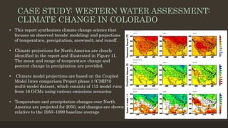
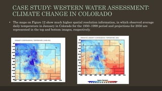
Params:
P7,D7,H7,A7
Region 7
Params:
P6,D6,H6,A6
Region 6
Params:
P5,D5,H5,A5
Region 5
Params:
P4,D4,H4,A4
Region 4
Params:
P3,D3,H3,A3
Region 3
Params:
P2,D2,H2,A2
Region 2
Params:
P1,D1,H1,A1
Region 1
Downscaling of data for climate projections
A Presentation by Submitted to
N.Nagadatt Sharma (191616) Prof K.V Jayakumar
Contents
• Introduction
• Impacts of Climate Change
• Global Climate Change Models
• Limitations of GCM’s
• Down scaling technics
• Types of downscaling
• Dynamic downscaling
• Statistical Downscaling
• Case study: western water assessment: climate change in Colorado
• Conclusion
• References
Introduction
• CLIMATE means “ average weather “. In general we consider the average condition of
conditions like temperature, rainfall, atmospheric pressure etc. for over 30 years.
What is weather ?
• General Definition: Any systematic change in the long term statistics of climate
elements (such as temperature, pressure, or winds) sustained over several decades or
longer.
• Climate is the average of long term observations of weather over a particular area
• Whereas weather is the day to day changes in the conditions over that area.
Climate and Weather
Impacts of climate change
• Global climate change has already had observable effects on the environment.
• Glaciers have shrunk, ice on rivers and lakes is breaking up earlier, plant and animal
ranges have shifted and trees are flowering sooner.
• Effects that scientists/researchers had predicted in the past as a result of global climate
change are now occurring: loss of sea ice, accelerated sea level rise and longer, more
intense heat waves, change in the seasons.
• Some of the future effects predicted are
• Continuous temperature rise
• Changes in precipitation patterns
Impacts of climate change
• More and severe droughts and heat
waves.
• Strong and Intense hurricanes
• Rise in sea-level by 1-4 feet by 2100
• Taken as a whole, the range of
published evidence indicates that the
net damage costs of climate change are
likely to be significant and to increase
over time
- Intergovernmental Panel on Climate Change
Global Climatic Models or
General or global circulation models (GCMs)
• General or global circulation models (GCMs) simulate the Earth’s climate via mathematical
equations that describe atmospheric, oceanic, and biotic processes, interactions, and
feedbacks.
• They are the primary tools that provide reasonably accurate global-, hemispheric-, and
continental-scale climate information and are used to understand present climate and
future climate scenarios under increased greenhouse gas concentrations.
• In each of the cells, GCMs compute the following: water vapor and cloud atmospheric
interactions, direct and indirect effects of aerosols on radiation and precipitation, changes
in snow cover and sea ice, the storage of heat in soils and oceans, surfaces fluxes of heat
and moisture, and large-scale transport of heat and water by the atmosphere and oceans
(Wilby et al., 2009).
General or global circulation models (GCMs)
• A GCM is composed of many grid cells
that represent horizontal and vertical
areas on the Earth’s surface (Figure).
• In summary, GCMs provide
quantitative estimates of future
climate change that are valid at the
global and continental scale and over
long periods.
Limitations of GCM’s
• Although GCMs are valuable predictive tools, they cannot account for fine-scale
heterogeneity of climate variability and change due to their coarse resolution.
• Numerous landscape features such as mountains, water bodies, infrastructure, land-
cover characteristics, and components of the climate system such as convective clouds
and coastal breezes, have scales that are much finer than 100–500 kilometers.
• Such heterogeneities are important for decision makers who require information on
potential impacts on crop production, hydrology, species distribution, etc. at scales of
10–50 kilometers.
• Often, global or continental-scale information is directly used to produce local-scale
impact maps, which is not appropriate since this large-scale information does not
account for differences at the local scale.
Down scaling Technics
• Various methods have been developed to bridge the gap between what GCMs can deliver
and what society/businesses/stakeholders require for decision making.
• The derivation of fine-scale climate information is based on the assumption that the local
climate is conditioned by interactions between large-scale atmospheric characteristics
(circulation, temperature, moisture, etc.) and local features (water bodies, mountain
ranges, land surface properties, etc.).
• In order to derive climate projections at scales that decision makers desire, a process
termed downscaling has been developed.
• It is possible to model these interactions and establish relationships between present-day
local climate and atmospheric conditions through the downscaling process
Down scaling Technics
• It is important to understand that the downscaling process
adds information to the coarse GCM output so that
information is more realistic at a finer scale, capturing sub-
grid scale contrasts and inhomogeneities
• The derivation of fine-scale climate information is based on
the assumption that the local climate is conditioned by
interactions between large-scale atmospheric
characteristics and local features
• It is possible to model these interactions and establish
relationships between present-day local climate and
atmospheric conditions through the downscaling process
Down scaling
Technics
Development of
Limited Area Models
(LAMs) ,(RCM’s) from
GCM’
Types of Downscaling
• Downscaling consists of a variety of methods, each with their own merits and limitations.
• Downscaling can be performed on spatial and temporal aspects of climate projections.
• Spatial downscaling refers to the methods used to derive finer-resolution spatial climate
information from coarser-resolution GCM output, e.g., 500 kilometers grid cell GCM output
to a 20 kilometers resolution, or even a specific location.
• Temporal downscaling refers to the derivation of fine-scale temporal information from
coarser-scale temporal GCM output (e.g., daily rainfall sequences from monthly or seasonal
rainfall amounts). Both approaches detailed below can be used to downscale monthly GCM
output to localized daily information.
Dynamic Downscaling
• Poor performances of GCMs at local and regional scales have lead to the development of
Limited Area Models (LAMs) in which a fine computational grid over a limited domain is
nested within the coarse grid of a GCM.
• This procedure is also known as DYNAMIC DOWNSCALING.
• Dynamical downscaling refers to the use of an RCM driven by a GCM to simulate regional
climate. An RCM is similar to a GCM but has higher resolution and additional regional
information, which enables it to better represent local landscape and possibly local
atmospheric processes.
• Most intensive downscaling studies and projects utilize various RCMs to produce a multi-
model ensemble and further validate results against observations.
Dynamic Downscaling
Advantages
• Based on consistent, physical mechanism
• Resolves atmospheric and surface processes occurring at sub-GCM grid scale
• Not constrained by historical record so that novel scenarios can be simulated
• Experiments involving an ensemble of RCMs are becoming available for uncertainty analysis
Disadvantages
• Computationally intensive
• Due to computational demands, RCMs are typically driven by only one or two GMC/emission scenario
simulations
• Limited number of RCMs available and no model results for many parts of the globe
• May require further downscaling and bias correction of RCM outputs
• Results depend on RCM assumptions; different RCMs will give different results
• Affected by bias of driving GCM
Statistical Downscaling
• Statistical downscaling involves the establishment of empirical relationships between
historical large-scale atmospheric and local climate characteristics.
• Once a relationship has been determined and validated, future large-scale atmospheric
conditions projected by GCMs are used to predict future local climate characteristics.
• In other words, large-scale GCM outputs are used as predictors5 to obtain local variables or
predictands. Statistical downscaling encompasses a heterogeneous group of methods that
vary in sophistication and applicability.
• Statistical downscaling methods are computationally inexpensive in comparison to RCMs
that require complex modeling of physical processes.
• Thus, they are a viable and sometimes advantageous alternative for institutions that do
not have the computational capacity and technical expertise required for dynamical
downscaling
Statistical Downscaling
• Although statistical downscaling is efficient, computationally inexpensive, and consists of a diverse
group of methods, it contains the following inherent assumptions:
1. The statistical relationship between the predictor and predictand does not change over time. .
2. The predictor carries the climate change signal.
3. There is a strong relationship between the predictor and predictand.
4. GCMs accurately simulate the predictor.
• Predictor validations are usually performed prior to a given GCM’s use in downscaling schemes.
• Statistical downscaling consists of a heterogeneous group of methods that vary in sophistication
and applicability
1. Linear methods
2. Weather classifications
3. Weather generators
Statistical Downscaling
Advantages
• Computationally inexpensive and efficient, which allows for many different emissions scenarios
and GCM pairings
• Methods range from simple to elaborate and are flexible enough to tailor for specific purposes
• The same method can be applied across regions or the entire globe, which facilitates comparisons
across different case studies
• Relies on the observed climate as a basis for driving future projections
• Can provide point-scale climatic variables for GCM-scale output
• Tools are freely available and easy to implement and interpret;
• some methods can capture extreme events
Disadvantages
• High quality observed data may be unavailable for many areas or variables
• Assumes that relationships between large and local-scale processes will remain the same in the
future (stationarity assumptions)
• The simplest methods may only provide projections at a monthly resolution
Applications
Dynamic downscaling
• Country or regional level (e.g.,
European Union) assessments with
significant government support and
resources
• Future planning by government
agencies across multiple sectors
• Impact studies that involve various
geographic areas
Statistical downscaling
• Weather generators in widespread use
for crop-yield, water, and other natural
resource modeling and management
• Delta or change factor method can be
applied for most adaptation activities
CASE STUDY: WESTERN WATER ASSESSMENT:
CLIMATE CHANGE IN COLORADO
• This report synthesizes climate change science that
focuses on observed trends; modeling; and projections
of temperature, precipitation, snowmelt, and runoff.
• Climate projections for North America are clearly
identified in the report and illustrated in Figure 11.
The mean and range of temperature change and
percent change in precipitation are provided.
• Climate model projections are based on the Coupled
Model Inter comparison Project phase 3 (CMIP3)
multi-model dataset, which consists of 112 model runs
from 16 GCMs using various emissions scenarios
• Temperature and precipitation changes over North
America are projected for 2050, and changes are shown
relative to the 1950–1999 baseline average
CASE STUDY: WESTERN WATER ASSESSMENT:
CLIMATE CHANGE IN COLORADO
• The maps on Figure 12 show much higher spatial resolution information, in which observed average
daily temperature in January in Colorado for the 1950–1999 period and projections for 2050 are
represented in the top and bottom images, respectively.
CASE STUDY: WESTERN WATER ASSESSMENT:
CLIMATE CHANGE IN COLORADO
• Observed climatological averages are taken from PRISM, a sophisticated climate mapping system
for the entire United States which incorporates point data, a digital elevation model, and expert
knowledge of complex climate systems to produce estimates of climate factors, e.g., temperature,
precipitation, etc
• PRISM is a mapping system that produces historical climate information. Projections were
downscaled and calculated via the delta method, in which the GCM multi-model average
temperature change was added to the observed climatology.
• Although PRISM is a legitimate dataset and the delta method is a commonly used downscaling
method the authors state that “temperature climatology does not capture year-to-year or day-to-
day variations and neither do the climate projections.”
• It is important to make the distinction that PRISM is not a predictive tool.
CONCLUSION
• The downscaling of global climate change projections has been developed to serve the needs of
decision makers who require local climate information for impact assessments.
• Downscaling to the order of 100–500 kilometers 10–50 kilometers is necessary for the assessment
of region- and station-scale climate information.
• GCM output can be downscaled via dynamical and/statistical means that vary in sophistication
and applicability.
• It is difficult to recommend which downscaling method is best, since the goals and resources of
each study are unique.
• Choosing the appropriate method depends on the user’s needs and can vary according to the
spatial and temporal resolution of the desired information and the climate variables that have the
highest impact on the region and/or sector being considered
Reference
• A review of downscaling methods for climate change projections
• Benestad, R. E. (2008). Empirical-Statistical Downscaling. Singapore: World Scientific
Publishing Co. Pte. Ltd
• Benestad, R. E. (2009). Downscaling precipitation extremes. Theoretical and Applied
Climatology 100(1-2), 1-2
• Various sites in the internet
Thank you
N.Nagadatt Sharma
Roll no 191616

Downscaling of global climate data.

  • 1.
    Params: P7,D7,H7,A7 Region 7 Params: P6,D6,H6,A6 Region 6 Params: P5,D5,H5,A5 Region5 Params: P4,D4,H4,A4 Region 4 Params: P3,D3,H3,A3 Region 3 Params: P2,D2,H2,A2 Region 2 Params: P1,D1,H1,A1 Region 1
  • 2.
    Downscaling of datafor climate projections A Presentation by Submitted to N.Nagadatt Sharma (191616) Prof K.V Jayakumar
  • 3.
    Contents • Introduction • Impactsof Climate Change • Global Climate Change Models • Limitations of GCM’s • Down scaling technics • Types of downscaling • Dynamic downscaling • Statistical Downscaling • Case study: western water assessment: climate change in Colorado • Conclusion • References
  • 4.
    Introduction • CLIMATE means“ average weather “. In general we consider the average condition of conditions like temperature, rainfall, atmospheric pressure etc. for over 30 years. What is weather ? • General Definition: Any systematic change in the long term statistics of climate elements (such as temperature, pressure, or winds) sustained over several decades or longer. • Climate is the average of long term observations of weather over a particular area • Whereas weather is the day to day changes in the conditions over that area.
  • 5.
  • 6.
    Impacts of climatechange • Global climate change has already had observable effects on the environment. • Glaciers have shrunk, ice on rivers and lakes is breaking up earlier, plant and animal ranges have shifted and trees are flowering sooner. • Effects that scientists/researchers had predicted in the past as a result of global climate change are now occurring: loss of sea ice, accelerated sea level rise and longer, more intense heat waves, change in the seasons. • Some of the future effects predicted are • Continuous temperature rise • Changes in precipitation patterns
  • 7.
    Impacts of climatechange • More and severe droughts and heat waves. • Strong and Intense hurricanes • Rise in sea-level by 1-4 feet by 2100 • Taken as a whole, the range of published evidence indicates that the net damage costs of climate change are likely to be significant and to increase over time - Intergovernmental Panel on Climate Change
  • 8.
    Global Climatic Modelsor General or global circulation models (GCMs) • General or global circulation models (GCMs) simulate the Earth’s climate via mathematical equations that describe atmospheric, oceanic, and biotic processes, interactions, and feedbacks. • They are the primary tools that provide reasonably accurate global-, hemispheric-, and continental-scale climate information and are used to understand present climate and future climate scenarios under increased greenhouse gas concentrations. • In each of the cells, GCMs compute the following: water vapor and cloud atmospheric interactions, direct and indirect effects of aerosols on radiation and precipitation, changes in snow cover and sea ice, the storage of heat in soils and oceans, surfaces fluxes of heat and moisture, and large-scale transport of heat and water by the atmosphere and oceans (Wilby et al., 2009).
  • 9.
    General or globalcirculation models (GCMs) • A GCM is composed of many grid cells that represent horizontal and vertical areas on the Earth’s surface (Figure). • In summary, GCMs provide quantitative estimates of future climate change that are valid at the global and continental scale and over long periods.
  • 10.
    Limitations of GCM’s •Although GCMs are valuable predictive tools, they cannot account for fine-scale heterogeneity of climate variability and change due to their coarse resolution. • Numerous landscape features such as mountains, water bodies, infrastructure, land- cover characteristics, and components of the climate system such as convective clouds and coastal breezes, have scales that are much finer than 100–500 kilometers. • Such heterogeneities are important for decision makers who require information on potential impacts on crop production, hydrology, species distribution, etc. at scales of 10–50 kilometers. • Often, global or continental-scale information is directly used to produce local-scale impact maps, which is not appropriate since this large-scale information does not account for differences at the local scale.
  • 11.
    Down scaling Technics •Various methods have been developed to bridge the gap between what GCMs can deliver and what society/businesses/stakeholders require for decision making. • The derivation of fine-scale climate information is based on the assumption that the local climate is conditioned by interactions between large-scale atmospheric characteristics (circulation, temperature, moisture, etc.) and local features (water bodies, mountain ranges, land surface properties, etc.). • In order to derive climate projections at scales that decision makers desire, a process termed downscaling has been developed. • It is possible to model these interactions and establish relationships between present-day local climate and atmospheric conditions through the downscaling process
  • 12.
    Down scaling Technics •It is important to understand that the downscaling process adds information to the coarse GCM output so that information is more realistic at a finer scale, capturing sub- grid scale contrasts and inhomogeneities • The derivation of fine-scale climate information is based on the assumption that the local climate is conditioned by interactions between large-scale atmospheric characteristics and local features • It is possible to model these interactions and establish relationships between present-day local climate and atmospheric conditions through the downscaling process
  • 13.
    Down scaling Technics Development of LimitedArea Models (LAMs) ,(RCM’s) from GCM’
  • 14.
    Types of Downscaling •Downscaling consists of a variety of methods, each with their own merits and limitations. • Downscaling can be performed on spatial and temporal aspects of climate projections. • Spatial downscaling refers to the methods used to derive finer-resolution spatial climate information from coarser-resolution GCM output, e.g., 500 kilometers grid cell GCM output to a 20 kilometers resolution, or even a specific location. • Temporal downscaling refers to the derivation of fine-scale temporal information from coarser-scale temporal GCM output (e.g., daily rainfall sequences from monthly or seasonal rainfall amounts). Both approaches detailed below can be used to downscale monthly GCM output to localized daily information.
  • 15.
    Dynamic Downscaling • Poorperformances of GCMs at local and regional scales have lead to the development of Limited Area Models (LAMs) in which a fine computational grid over a limited domain is nested within the coarse grid of a GCM. • This procedure is also known as DYNAMIC DOWNSCALING. • Dynamical downscaling refers to the use of an RCM driven by a GCM to simulate regional climate. An RCM is similar to a GCM but has higher resolution and additional regional information, which enables it to better represent local landscape and possibly local atmospheric processes. • Most intensive downscaling studies and projects utilize various RCMs to produce a multi- model ensemble and further validate results against observations.
  • 16.
    Dynamic Downscaling Advantages • Basedon consistent, physical mechanism • Resolves atmospheric and surface processes occurring at sub-GCM grid scale • Not constrained by historical record so that novel scenarios can be simulated • Experiments involving an ensemble of RCMs are becoming available for uncertainty analysis Disadvantages • Computationally intensive • Due to computational demands, RCMs are typically driven by only one or two GMC/emission scenario simulations • Limited number of RCMs available and no model results for many parts of the globe • May require further downscaling and bias correction of RCM outputs • Results depend on RCM assumptions; different RCMs will give different results • Affected by bias of driving GCM
  • 17.
    Statistical Downscaling • Statisticaldownscaling involves the establishment of empirical relationships between historical large-scale atmospheric and local climate characteristics. • Once a relationship has been determined and validated, future large-scale atmospheric conditions projected by GCMs are used to predict future local climate characteristics. • In other words, large-scale GCM outputs are used as predictors5 to obtain local variables or predictands. Statistical downscaling encompasses a heterogeneous group of methods that vary in sophistication and applicability. • Statistical downscaling methods are computationally inexpensive in comparison to RCMs that require complex modeling of physical processes. • Thus, they are a viable and sometimes advantageous alternative for institutions that do not have the computational capacity and technical expertise required for dynamical downscaling
  • 18.
    Statistical Downscaling • Althoughstatistical downscaling is efficient, computationally inexpensive, and consists of a diverse group of methods, it contains the following inherent assumptions: 1. The statistical relationship between the predictor and predictand does not change over time. . 2. The predictor carries the climate change signal. 3. There is a strong relationship between the predictor and predictand. 4. GCMs accurately simulate the predictor. • Predictor validations are usually performed prior to a given GCM’s use in downscaling schemes. • Statistical downscaling consists of a heterogeneous group of methods that vary in sophistication and applicability 1. Linear methods 2. Weather classifications 3. Weather generators
  • 19.
    Statistical Downscaling Advantages • Computationallyinexpensive and efficient, which allows for many different emissions scenarios and GCM pairings • Methods range from simple to elaborate and are flexible enough to tailor for specific purposes • The same method can be applied across regions or the entire globe, which facilitates comparisons across different case studies • Relies on the observed climate as a basis for driving future projections • Can provide point-scale climatic variables for GCM-scale output • Tools are freely available and easy to implement and interpret; • some methods can capture extreme events Disadvantages • High quality observed data may be unavailable for many areas or variables • Assumes that relationships between large and local-scale processes will remain the same in the future (stationarity assumptions) • The simplest methods may only provide projections at a monthly resolution
  • 20.
    Applications Dynamic downscaling • Countryor regional level (e.g., European Union) assessments with significant government support and resources • Future planning by government agencies across multiple sectors • Impact studies that involve various geographic areas Statistical downscaling • Weather generators in widespread use for crop-yield, water, and other natural resource modeling and management • Delta or change factor method can be applied for most adaptation activities
  • 21.
    CASE STUDY: WESTERNWATER ASSESSMENT: CLIMATE CHANGE IN COLORADO • This report synthesizes climate change science that focuses on observed trends; modeling; and projections of temperature, precipitation, snowmelt, and runoff. • Climate projections for North America are clearly identified in the report and illustrated in Figure 11. The mean and range of temperature change and percent change in precipitation are provided. • Climate model projections are based on the Coupled Model Inter comparison Project phase 3 (CMIP3) multi-model dataset, which consists of 112 model runs from 16 GCMs using various emissions scenarios • Temperature and precipitation changes over North America are projected for 2050, and changes are shown relative to the 1950–1999 baseline average
  • 22.
    CASE STUDY: WESTERNWATER ASSESSMENT: CLIMATE CHANGE IN COLORADO • The maps on Figure 12 show much higher spatial resolution information, in which observed average daily temperature in January in Colorado for the 1950–1999 period and projections for 2050 are represented in the top and bottom images, respectively.
  • 23.
    CASE STUDY: WESTERNWATER ASSESSMENT: CLIMATE CHANGE IN COLORADO • Observed climatological averages are taken from PRISM, a sophisticated climate mapping system for the entire United States which incorporates point data, a digital elevation model, and expert knowledge of complex climate systems to produce estimates of climate factors, e.g., temperature, precipitation, etc • PRISM is a mapping system that produces historical climate information. Projections were downscaled and calculated via the delta method, in which the GCM multi-model average temperature change was added to the observed climatology. • Although PRISM is a legitimate dataset and the delta method is a commonly used downscaling method the authors state that “temperature climatology does not capture year-to-year or day-to- day variations and neither do the climate projections.” • It is important to make the distinction that PRISM is not a predictive tool.
  • 24.
    CONCLUSION • The downscalingof global climate change projections has been developed to serve the needs of decision makers who require local climate information for impact assessments. • Downscaling to the order of 100–500 kilometers 10–50 kilometers is necessary for the assessment of region- and station-scale climate information. • GCM output can be downscaled via dynamical and/statistical means that vary in sophistication and applicability. • It is difficult to recommend which downscaling method is best, since the goals and resources of each study are unique. • Choosing the appropriate method depends on the user’s needs and can vary according to the spatial and temporal resolution of the desired information and the climate variables that have the highest impact on the region and/or sector being considered
  • 25.
    Reference • A reviewof downscaling methods for climate change projections • Benestad, R. E. (2008). Empirical-Statistical Downscaling. Singapore: World Scientific Publishing Co. Pte. Ltd • Benestad, R. E. (2009). Downscaling precipitation extremes. Theoretical and Applied Climatology 100(1-2), 1-2 • Various sites in the internet Thank you N.Nagadatt Sharma Roll no 191616