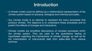
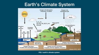
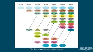
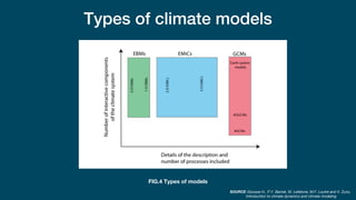
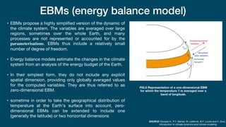
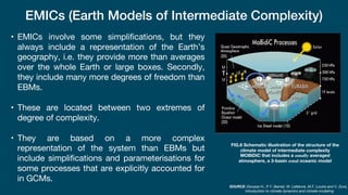
Models in Climate Science
Submitted by-
Adarsh Singh (2K19/ENE/07)
M.TECH 1st year Environmental Engineering
Delhi Technological University
1
Introduction
• A climate model could be defined as a mathematical representation of the
climate system based on physical, biological and chemical principles .
• Any climate model is an attempt to represent the many processes that
produce climate. The objective is to understand these processes and to
predict the effects of changes and interactions.
• Climate models are simplified descriptions of complex processes within
the climate system. They are used for the quantitative testing of
hypotheses regarding the mechanisms of climate change, as well as for
the interpretation of instrumental data from paleo-data from various
archives.
Earth’s Climate System
FIG.1 earth’s climate system
Important components of climate model
1. solar radiation (absorbed by atmosphere and sea)
2. Dynamics (eg. movement of energy/heats and mass)
3. Surface Processes (effects of ice, snow, vegetation and moisture
interchanges)
4. Chemistry (chemical composition of atmosphere)
5. Resolution in both time and space (the time step of model and horizontal
and vertical scale resolve)
Source:McGuffie and Henderson-sellers,Climate modelling Primer,3rd edition
Model development
FIG.2 Schematic representation of the development and use of a climate model.
SOURCE :Goosse H., P.Y.
Barriat, W. Lefebvre, M.F.
Loutre and V. Zunz,
Introduction to climate
dynamics and climate
modeling
An energy balance model based on E=𝜎𝑇!
Let, initial condition be
No sun ,Earth temperature -> 32K (−241!
𝐶)
emits-> 0.06𝑤/𝑚!
Case 1-No reflection
No GHG
Inflow
=341𝑤/𝑚!
Absorbed
=341𝑤/𝑚!
Initial outflow
=0.06𝑤/𝑚!
Grows to
=341𝑤/𝑚!
temperature gradually
increase to 278K
(5!
𝐶)
Case 2- Add reflection
No GHG
Inflow
=341𝑤/𝑚!
Absorbed
=239𝑤/𝑚!
Emitted
=239𝑤/𝑚!
reflected
=102𝑤/𝑚!
(30%)
temperature cools
down from 5!
𝐶 to
− 18"𝐶
Inflow
=341𝑤/𝑚!
Absorbed
=239𝑤/𝑚!
reflected
=102𝑤/𝑚!
(30%)
temperature warms
up to 30"𝐶
Case 3- Add GHG
earth emission
absorbed in
atmosphere
239𝑤/𝑚!
239𝑤/𝑚!
478𝑤/𝑚!
Source: UBC online course on climate literacy
FIG.3 Chronology of climate model development
SOURCE :figure modified
from IPCC (2001), Technical
Summary (Box 3, Figure 1, p.
48)
Types of climate models
SOURCE :Goosse H., P.Y. Barriat, W. Lefebvre, M.F. Loutre and V. Zunz,
Introduction to climate dynamics and climate modeling
FIG.4 Types of models
EBMs (energy balance model)
• EBMs propose a highly simplified version of the dynamic of
the climate system. The variables are averaged over large
regions, sometimes over the whole Earth, and many
processes are not represented or accounted for by the
parameterisations. EBMs thus include a relatively small
number of degree of freedom.
• Energy balance models estimate the changes in the climate
system from an analysis of the energy budget of the Earth.
• In their simplest form, they do not include any explicit
spatial dimension, providing only globally averaged values
for the computed variables. They are thus referred to as
zero-dimensional EBM.
• sometime in order to take the geographical distribution of
temperature at the Earth’s surface into account, zero-
dimensional EBMs can be extended to include one
(generally the latitude) or two horizontal dimensions
FIG.5 Representation of a one-dimensional EBM
for which the temperature Ti is averaged over a
band of longitude.
SOURCE :Goosse H., P.Y. Barriat, W. Lefebvre, M.F. Loutre and V. Zunz,
Introduction to climate dynamics and climate modeling
EMICs (Earth Models of Intermediate Complexity)
• EMICs involve some simplifications, but they
always include a representation of the Earth’s
geography, i.e. they provide more than averages
over the whole Earth or large boxes. Secondly,
they include many more degrees of freedom than
EBMs.
• These are located between two extremes of
degree of complexity.
• They are based on a more complex
representation of the system than EBMs but
include simplifications and parameterisations for
some processes that are explicitly accounted for
in GCMs.
SOURCE :Goosse H., P.Y. Barriat, W. Lefebvre, M.F. Loutre and V. Zunz,
Introduction to climate dynamics and climate modeling
FIG.6 Schematic illustration of the structure of the
climate model of intermediate complexity
MOBIDIC that includes a zonally averaged
atmosphere, a 3-basin zonal oceanic model
GCMs (general circulation model)
• General circulation models provide the most precise and complex description of the climate system.
GCMs divide the globe into a three-dimensional grid of cells representing specific geographic locations
and elevations. Each of the components has equations calculated on the global grid for a set of climate
variables such as temperature.
• In addition to model components computing how they are changing over time, the different parts
exchange fluxes of heat, water, and momentum. They interact with one another as a coupled system.
• Their grid resolution is typically of the order of 100 to 200 km. As a result , compared to EMICs (which
have a grid resolution between 300 km and thousands of kilometres), they provide much more detailed
information on a regional scale.
• earlierGCMs only included a representation of the atmosphere, the land surface, sometimes the ocean
circulation, and a very simplified version of the sea ice. Nowadays, GCMs take more and more
components into account like sophisticated models of the sea ice, the carbon cycle, ice sheet dynamics
and even atmospheric chemistry.
• Because of the large number of processes included and their relatively high resolution, GCM simulations
require a large amount of computer time.
FIG.7 A simplified representation of part of the domain of a general circulation model, illustrating some important
components and processes. SOURCE :Goosse H., P.Y. Barriat, W. Lefebvre, M.F. Loutre and V. Zunz,
Introduction to climate dynamics and climate modeling
Grid Size
• Grid size depend on power of computer.
• finer resolution implies a larger number of
grid cells and requires a bigger and faster
computer to perform the simulation.
• if grid spacing is farther apart, there are
fewer points that are calculated, but the
results are also less detailed.
• Simulated model are larger than grid scale
and based on bedrock scientific principles
eg. cyclone
• Parameterized processes represent more
complex processes that are smaller than
grid scale eg. cloud and aerosol
source
https://www.gfdl.noaa.gov/climate-modeling/
observed
data
provided
by
Prism
climate
group,
Oregon
state
university
Virtual time and computational cost
10 years
1000 years
100 years
• These are most complex models
• Highest Resolutions
• most things to keep track of
• These are relevant for current human generation i.e. human lifetime
• answers question like what will be impact of all GHGs emission in
century
• These models are tested against geological
observations
• adresses future questions like fate of long term
GHG emission, how long will it take to melt ice on
Greenland
• Computational costs
Time to run your model = Computer time to run each math operations
X # of math operations per equations
X # of equations per grid cells
X # of grid cell in model
X # total time steps
X # of model runs
Drawbacks of Model Complexity
• A more complex model doesn’t mean more reliable.
• A complex model may be more realistic yet ironically as we add more factors to
it the certainty of its prediction may decrease even as our intuitive faith in our
model increases.
• Climate models are not exact replicas of climate systems instead they are
useful tools for learning which required continuous checks.
Models output
SOURCE :IPCC 2007
Climate Change 2007: Working Group I: The Physical Science Basis
Temperature anomaly observations
since 1900 i.e. measured temperature
outputs from climate models (there are
58 different yellow lines and
model runs from 14 different models)
Average of all yellow lines
•Checking against observations
SOURCE :IPCC 2007
Climate Change 2007: Working Group I: The Physical Science Basis
• Models help with attribution
Temperature with observations
Modeled temperature
with human activities
Temperature with observations
Modeled temperature without human activities
• Checking prediction
SOURCE : Copenhagen Diagnosis 2009
FIG.8 Sea level change during 1970-2010. The tide gauge data are indicated in red (Church
and White 2006) and satellite data in blue (Cazenave et al. 2008).The grey band shows the
projections of the IPCC Third Assessment report for comparison
•Predicting future
• two approaches SRES (special report on emission scenarios) and RCPs
approach (representative concentration pathways) are used to predict future
1.SRES Approach
(storyline approach)
FIG.9 Schematic of SRES family
SOURCE :IPCC 2007 report
2. RCP Approach
• A Representative Concentration Pathway (RCP) is a greenhouse
gas concentration (not emissions) trajectory adopted by the IPCC.
• Four pathways were used for climate modeling and research for the IPCC AR5.
• These are four: RCP8.5, RCP6, RCP4.5, and RCP2.6 (also referred to as
RCP3PD, where 'PD' stands for Peak and Decline). The numbers refer to
radiative forcing measured in watts per square metre, by the year 2100.
Source: IPCC AR5
DATA: MEINHAUSENET AL 2011
REFERENCES
• IPCC AR4 WG1 (2007), Climate Change 2007: The Physical Science Basis, Contribution of Working
Group I to the Fourth Assessment Report of the Intergovernmental Panel on Climate Change
• IPCC AR 5 (2014), climate Change 2014
• McGuffie and Henderson-sellers,Climate modelling Primer,3rd edition
• Goosse H., P.Y. Barriat, W. Lefebvre, M.F. Loutre and V. Zunz, Introduction to climate dynamics and
climate modelling
THANK
YOU

Models in climate science

  • 1.
    Models in ClimateScience Submitted by- Adarsh Singh (2K19/ENE/07) M.TECH 1st year Environmental Engineering Delhi Technological University 1
  • 2.
    Introduction • A climatemodel could be defined as a mathematical representation of the climate system based on physical, biological and chemical principles . • Any climate model is an attempt to represent the many processes that produce climate. The objective is to understand these processes and to predict the effects of changes and interactions. • Climate models are simplified descriptions of complex processes within the climate system. They are used for the quantitative testing of hypotheses regarding the mechanisms of climate change, as well as for the interpretation of instrumental data from paleo-data from various archives.
  • 3.
    Earth’s Climate System FIG.1earth’s climate system
  • 4.
    Important components ofclimate model 1. solar radiation (absorbed by atmosphere and sea) 2. Dynamics (eg. movement of energy/heats and mass) 3. Surface Processes (effects of ice, snow, vegetation and moisture interchanges) 4. Chemistry (chemical composition of atmosphere) 5. Resolution in both time and space (the time step of model and horizontal and vertical scale resolve) Source:McGuffie and Henderson-sellers,Climate modelling Primer,3rd edition
  • 5.
    Model development FIG.2 Schematicrepresentation of the development and use of a climate model. SOURCE :Goosse H., P.Y. Barriat, W. Lefebvre, M.F. Loutre and V. Zunz, Introduction to climate dynamics and climate modeling
  • 6.
    An energy balancemodel based on E=𝜎𝑇! Let, initial condition be No sun ,Earth temperature -> 32K (−241! 𝐶) emits-> 0.06𝑤/𝑚! Case 1-No reflection No GHG Inflow =341𝑤/𝑚! Absorbed =341𝑤/𝑚! Initial outflow =0.06𝑤/𝑚! Grows to =341𝑤/𝑚! temperature gradually increase to 278K (5! 𝐶) Case 2- Add reflection No GHG Inflow =341𝑤/𝑚! Absorbed =239𝑤/𝑚! Emitted =239𝑤/𝑚! reflected =102𝑤/𝑚! (30%) temperature cools down from 5! 𝐶 to − 18"𝐶 Inflow =341𝑤/𝑚! Absorbed =239𝑤/𝑚! reflected =102𝑤/𝑚! (30%) temperature warms up to 30"𝐶 Case 3- Add GHG earth emission absorbed in atmosphere 239𝑤/𝑚! 239𝑤/𝑚! 478𝑤/𝑚! Source: UBC online course on climate literacy
  • 7.
    Source: UBC onlinecourse on climate literacy
  • 8.
    FIG.3 Chronology ofclimate model development SOURCE :figure modified from IPCC (2001), Technical Summary (Box 3, Figure 1, p. 48)
  • 9.
    Types of climatemodels SOURCE :Goosse H., P.Y. Barriat, W. Lefebvre, M.F. Loutre and V. Zunz, Introduction to climate dynamics and climate modeling FIG.4 Types of models
  • 10.
    EBMs (energy balancemodel) • EBMs propose a highly simplified version of the dynamic of the climate system. The variables are averaged over large regions, sometimes over the whole Earth, and many processes are not represented or accounted for by the parameterisations. EBMs thus include a relatively small number of degree of freedom. • Energy balance models estimate the changes in the climate system from an analysis of the energy budget of the Earth. • In their simplest form, they do not include any explicit spatial dimension, providing only globally averaged values for the computed variables. They are thus referred to as zero-dimensional EBM. • sometime in order to take the geographical distribution of temperature at the Earth’s surface into account, zero- dimensional EBMs can be extended to include one (generally the latitude) or two horizontal dimensions FIG.5 Representation of a one-dimensional EBM for which the temperature Ti is averaged over a band of longitude. SOURCE :Goosse H., P.Y. Barriat, W. Lefebvre, M.F. Loutre and V. Zunz, Introduction to climate dynamics and climate modeling
  • 11.
    EMICs (Earth Modelsof Intermediate Complexity) • EMICs involve some simplifications, but they always include a representation of the Earth’s geography, i.e. they provide more than averages over the whole Earth or large boxes. Secondly, they include many more degrees of freedom than EBMs. • These are located between two extremes of degree of complexity. • They are based on a more complex representation of the system than EBMs but include simplifications and parameterisations for some processes that are explicitly accounted for in GCMs. SOURCE :Goosse H., P.Y. Barriat, W. Lefebvre, M.F. Loutre and V. Zunz, Introduction to climate dynamics and climate modeling FIG.6 Schematic illustration of the structure of the climate model of intermediate complexity MOBIDIC that includes a zonally averaged atmosphere, a 3-basin zonal oceanic model
  • 12.
    GCMs (general circulationmodel) • General circulation models provide the most precise and complex description of the climate system. GCMs divide the globe into a three-dimensional grid of cells representing specific geographic locations and elevations. Each of the components has equations calculated on the global grid for a set of climate variables such as temperature. • In addition to model components computing how they are changing over time, the different parts exchange fluxes of heat, water, and momentum. They interact with one another as a coupled system. • Their grid resolution is typically of the order of 100 to 200 km. As a result , compared to EMICs (which have a grid resolution between 300 km and thousands of kilometres), they provide much more detailed information on a regional scale. • earlierGCMs only included a representation of the atmosphere, the land surface, sometimes the ocean circulation, and a very simplified version of the sea ice. Nowadays, GCMs take more and more components into account like sophisticated models of the sea ice, the carbon cycle, ice sheet dynamics and even atmospheric chemistry. • Because of the large number of processes included and their relatively high resolution, GCM simulations require a large amount of computer time.
  • 13.
    FIG.7 A simplifiedrepresentation of part of the domain of a general circulation model, illustrating some important components and processes. SOURCE :Goosse H., P.Y. Barriat, W. Lefebvre, M.F. Loutre and V. Zunz, Introduction to climate dynamics and climate modeling
  • 14.
    Grid Size • Gridsize depend on power of computer. • finer resolution implies a larger number of grid cells and requires a bigger and faster computer to perform the simulation. • if grid spacing is farther apart, there are fewer points that are calculated, but the results are also less detailed. • Simulated model are larger than grid scale and based on bedrock scientific principles eg. cyclone • Parameterized processes represent more complex processes that are smaller than grid scale eg. cloud and aerosol source https://www.gfdl.noaa.gov/climate-modeling/ observed data provided by Prism climate group, Oregon state university
  • 15.
    Virtual time andcomputational cost 10 years 1000 years 100 years • These are most complex models • Highest Resolutions • most things to keep track of • These are relevant for current human generation i.e. human lifetime • answers question like what will be impact of all GHGs emission in century • These models are tested against geological observations • adresses future questions like fate of long term GHG emission, how long will it take to melt ice on Greenland
  • 16.
    • Computational costs Timeto run your model = Computer time to run each math operations X # of math operations per equations X # of equations per grid cells X # of grid cell in model X # total time steps X # of model runs
  • 17.
    Drawbacks of ModelComplexity • A more complex model doesn’t mean more reliable. • A complex model may be more realistic yet ironically as we add more factors to it the certainty of its prediction may decrease even as our intuitive faith in our model increases. • Climate models are not exact replicas of climate systems instead they are useful tools for learning which required continuous checks.
  • 18.
    Models output SOURCE :IPCC2007 Climate Change 2007: Working Group I: The Physical Science Basis Temperature anomaly observations since 1900 i.e. measured temperature outputs from climate models (there are 58 different yellow lines and model runs from 14 different models) Average of all yellow lines •Checking against observations
  • 19.
    SOURCE :IPCC 2007 ClimateChange 2007: Working Group I: The Physical Science Basis • Models help with attribution Temperature with observations Modeled temperature with human activities Temperature with observations Modeled temperature without human activities
  • 20.
    • Checking prediction SOURCE: Copenhagen Diagnosis 2009 FIG.8 Sea level change during 1970-2010. The tide gauge data are indicated in red (Church and White 2006) and satellite data in blue (Cazenave et al. 2008).The grey band shows the projections of the IPCC Third Assessment report for comparison
  • 21.
    •Predicting future • twoapproaches SRES (special report on emission scenarios) and RCPs approach (representative concentration pathways) are used to predict future 1.SRES Approach (storyline approach)
  • 22.
    FIG.9 Schematic ofSRES family
  • 23.
  • 24.
    2. RCP Approach •A Representative Concentration Pathway (RCP) is a greenhouse gas concentration (not emissions) trajectory adopted by the IPCC. • Four pathways were used for climate modeling and research for the IPCC AR5. • These are four: RCP8.5, RCP6, RCP4.5, and RCP2.6 (also referred to as RCP3PD, where 'PD' stands for Peak and Decline). The numbers refer to radiative forcing measured in watts per square metre, by the year 2100.
  • 25.
    Source: IPCC AR5 DATA:MEINHAUSENET AL 2011
  • 26.
    REFERENCES • IPCC AR4WG1 (2007), Climate Change 2007: The Physical Science Basis, Contribution of Working Group I to the Fourth Assessment Report of the Intergovernmental Panel on Climate Change • IPCC AR 5 (2014), climate Change 2014 • McGuffie and Henderson-sellers,Climate modelling Primer,3rd edition • Goosse H., P.Y. Barriat, W. Lefebvre, M.F. Loutre and V. Zunz, Introduction to climate dynamics and climate modelling
  • 27.