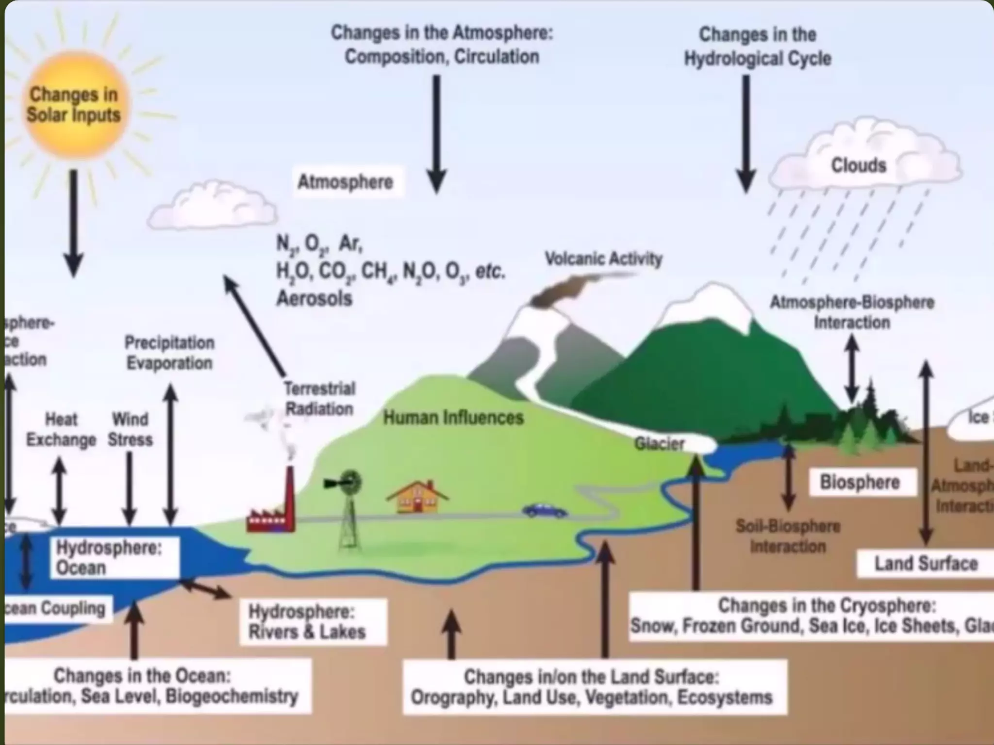
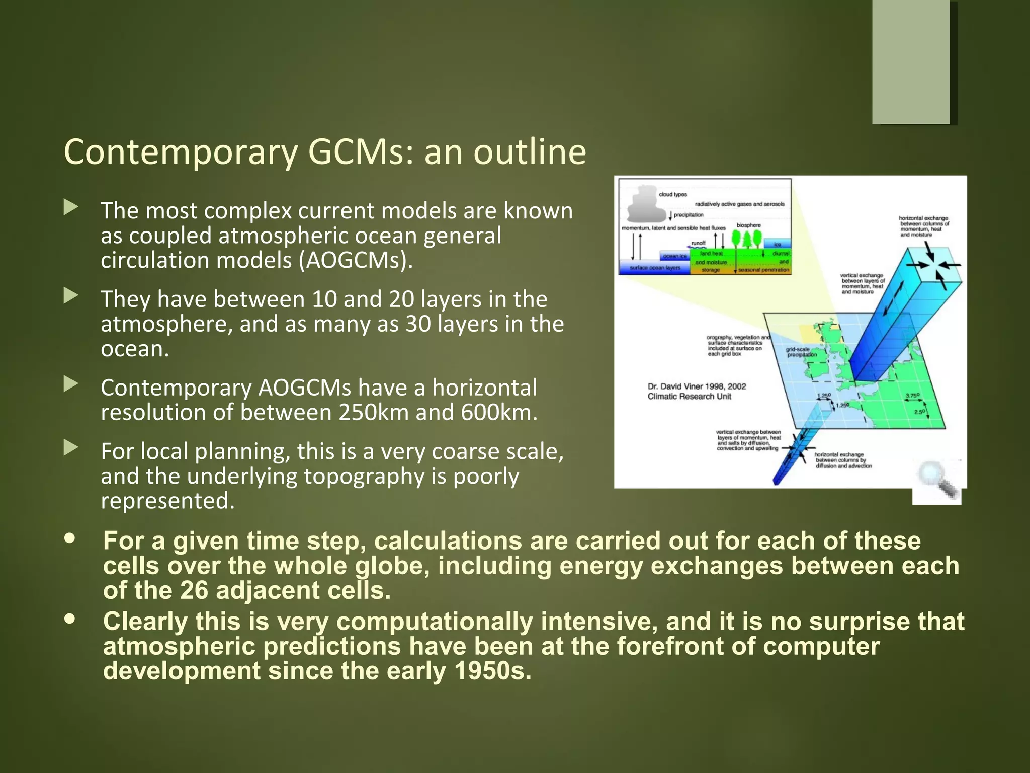
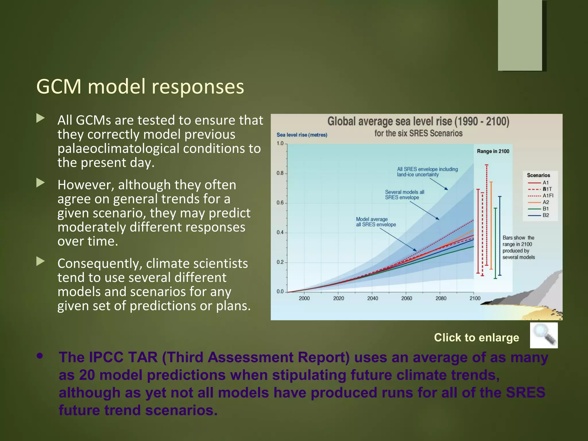
General circulation
Model
Contents:
• DEFINITION OF MODEL & GCM…
• FACTORS OF GCM…
• NWP VS CLIMATE MODELS…
• HOW CLIMATE WORKS…
• TYPES OF GCM…
• WORKING OF GCM…
• USES , EFFECTS & CONCLUSION…
MODEL;
Smaller representation of a larger object.
GCM;
A computer model that both identifies possible causes of
climate change & predicts climate change into Future.
1;Living organism.
2;Glacier ice.
3;ENERGY FROM SUN.
4;LAND FORMS
5;HOW ALL THESE FACTORS
INTERACT.
FACTORS OF GCMFACTORS OF GCM
Different types of climate models
 It is often convenient to regard climate models as
belonging to one of four main categories:
 energy balance models (EBMs)
 one dimensional radiative-convective models (RCMs);
 two-dimensional statistical-dynamical models (SDMs)
 three-dimensional general circulation models (GCMs).
 It is not always necessary to use the most complex model.
 Using a simpler model allows more runs to be carried out
as sensitivity tests to assess the accuracy of modelling
assumptions.
Global circulation models
 GCMs “…are the only credible tools currently available for
simulating the response of the global climate system to
increasing greenhouse gas concentrations” (IPCC-TGCIA, 1999).
 The first GCM was a very simple 2 layer, hemispheric, quasi-
geotrophic computer model, developed in the 1950’s by
Norman Philips.
 Such early GCMs involved several atmospheric layers and a
very simple oceanic model. The model was run to equilibrium
with a set CO2 level (such as 300ppm) and then the CO2 level
was increased.
 Contemporary models are considerably more complex, and are
capable of being run in a transient mode.
 They are 3-D, and may comprise thousands of individual cells
Contemporary GCMs: an outline
 The most complex current models are known
as coupled atmospheric ocean general
circulation models (AOGCMs).
 They have between 10 and 20 layers in the
atmosphere, and as many as 30 layers in the
ocean.
 Contemporary AOGCMs have a horizontal
resolution of between 250km and 600km.
 For local planning, this is a very coarse scale,
and the underlying topography is poorly
represented.
 For a given time step, calculations are carried out for each of these
cells over the whole globe, including energy exchanges between each
of the 26 adjacent cells.
 Clearly this is very computationally intensive, and it is no surprise that
atmospheric predictions have been at the forefront of computer
development since the early 1950s.
Climatic processes modelled in a GCM
Thermodynamic
equation
Equation of
motion
Radiation
transfer
Equation of
water vapour
Heat balance Hydrology
of the earth’s surface
DENSITY
ADVECTION
ADVECTION
HEAT OFCONDENSATION
MOISTURE
HEATINGAND
COOLING
HEAT ENERGY
EVAPO
RATIO
N
SNOW
COVER
FEEDBACK
PRECIPITATION
Flux adjustments
 Some GCMs do not correctly provide a stable equilibrium
condition under current climatic conditions.
 In order to ensure they accurately do so, a number of “flux
adjustments” are provided.
 These are non-physical correction constants that are used as
correction factors to ensure that the models stay on track.
 More recently, through intensive exploration of more exacting
physical calculations, some models have been developed that
do not flux adjustments.
 Some non-flux adjusted models are now able to maintain
stable climatologies of comparable quality to flux adjusted
models.
 Furthermore, there is no systematic difference between the
outputs of flux-adjusted and non-flux-adjusted models in
terms of internal climatic variability.
How many GCMs are there?
 Considering the incredible computing power necessary to run
a full GCM, one would expect there to be only a few models.
 In fact, a number of different groups have developed and
refined models over the years, and the IPCC Third Assessment
Report uses no fewer than 34 AOGCMs, some of which exist in
several refinements.
 These models are developed and operated by 18 different
climatology centres, including the UK Meteorological Centre,
National Center for Atmospheric Research,
Goddard Institute for Space Studies and the
Geophysical Fluid Dynamics Laboratory.
 These models are run nearly constantly, and the results are
published on the internet in order to allow planners and
response modellers ready access.
Use of GCMs
 GCMs enable us to better understand the
processes that drive the climate. Models
that work better at describing climatic
conditions generally give us an insight into
how the various physical characteristics of
the earth are interacting.
 They allow us to make informed and
scientifically defensible predictions based
on current understanding of the climate.
 GCMs are thus the best tools for all climate
science, and allow conservationists,
planners and politicians to test different
response scenarios.
The effects of current radiative forcings
Source:
IPCC online
slide
archive
IPCC future scenarios
 In order to predict future climate responses, the IPCC has
modelled and detailed several different scenarios (IPCC, 1992;
IPCC, 2000).
 The SRES scenarios fall into four main “storyline” categories.
 A1 – rapid economic growth and introduction of efficient
technologies.
- Global population peaks mid-century, then decreases.
- Global capacity building; difference in per capita income between
regions decreases.
- Three separate sub scenarios depending on energy policy:
• A1FI – fossil fuel intensive.
• A1T – fossil fuel use phased out entirely.
• A1B – balanced use of all sources ( no one dominates).
Development scenarios (cont).
 A2 – very heterogenous world, focussed on self- reliance.
 Constant population growth due to slow fertility rate change
 Per capita economic and technological growth slow
 Regional responses
 B1 – similar population growth and global economy to scenario A1.
 Rapid transition to service economies (low-impact)
 Focus on provision of clean, resource efficient technology.
 Global solutions to economic inequities, but no other climate
initiatives.
 B2 – emphasis on local solutions to economic, social, and environmental
sustainability
 Constant population growth (slower than A2).
 Slower economic/social growth, focussed on a regional scale.
 Focussed on environmental solutions and greater equity, but on a
regional rather than global scale.
Future radiative forcings depend on response
 Current climate change is largely
anthropogenic in origin.
 Human activities are likely to
continue to affect the climate in
a similar manner.
 Consequently, the human
political and economic response
to global climate change is
essential.
 The SRES scenarios demonstrate
how human response is likely to
affect global greenhouse gas
and aerosol emissions.
Source: IPCC online slides
GCM model responses
 All GCMs are tested to ensure that
they correctly model previous
palaeoclimatological conditions to
the present day.
 However, although they often
agree on general trends for a
given scenario, they may predict
moderately different responses
over time.
 Consequently, climate scientists
tend to use several different
models and scenarios for any
given set of predictions or plans.
 The IPCC TAR (Third Assessment Report) uses an average of as many
as 20 model predictions when stipulating future climate trends,
although as yet not all models have produced runs for all of the SRES
future trend scenarios.
Click to enlarge
GCM outputs for 2100 (I)
Source: IPCC
online slides
(SYR fig 3-3a &b)
GCM outputs for 2100 (II)
Linear and non linear responses
 Many climatic responses to changing conditions are linear in nature
(either logarithmically through feedback mechanisms or as a flat line).
 However, palaeoclimatological evidence points towards a number of
periods of extremely rapid climate change.
 This is typical of non-linear systems with multiple stable equilibria (Lorenz,
1993).
 When conditions are pushed towards a “threshold value”, the transition
to a new mode may be exceedingly rapid.
 This has also been seen in recent changes in large scale circulation
patterns detected by instrumental readings, and in contemporary
observations of regional weather patterns. (Corti et al, 1999).
Examples of non-linear changes
 Most GCMs show a slowing of the Atlantic Thermohaline Circulation as the world
heats up. However, some show the circulation stopping entirely as heating reaches
a threshold value. (Manabe and Stouffer, 1988).
 Sea ice melting may be accelerated by feedback mechanisms.
 Sea level rise may destabilise large polar ice masses, ice sheets, or even entire ice
shelves, accelerating sea level rise.
 Observed variability of ENSO indicate a transition to increased occurrence of ENSO
in 1976, although not enough is know to say whether this is an anthropogenic
effect, or even if it is a long-term transition.
 Large-scale (possibly irreversible) transformations in the biosphere such as the
growth of the Sahara desert (Claussen et al., 1999), have occurred even with minimal
anthropogenic interaction. These can be seen as non-linear changes triggered by
slow changes in forcing factors, and it seems highly possible that this could occur
given the current level of anthropogenic disturbance. However, not enough is
know about this incredibly complex system to say this with any degree of
certainty.
Conclusion
 General circulation models are the best
tool we have for determining the range
and extent of climate change, as well as
for working out what is likely to happen
in the future.
 All current models agree that current
climatic change is a result of
anthropogenic influences.
 Future climate change will depend on the
current human response to that
knowledge.
 Although GCM outputs are very large
scale, they can be refined and
downscaled to assist in prediction for
smaller areas.
 Thus, the outputs from GCMs can be
exceedingly useful in terms of
conservation planning for responses to
climate change.

General circulation model

  • 1.
  • 2.
    Contents: • DEFINITION OFMODEL & GCM… • FACTORS OF GCM… • NWP VS CLIMATE MODELS… • HOW CLIMATE WORKS… • TYPES OF GCM… • WORKING OF GCM… • USES , EFFECTS & CONCLUSION…
  • 3.
    MODEL; Smaller representation ofa larger object. GCM; A computer model that both identifies possible causes of climate change & predicts climate change into Future.
  • 4.
    1;Living organism. 2;Glacier ice. 3;ENERGYFROM SUN. 4;LAND FORMS 5;HOW ALL THESE FACTORS INTERACT. FACTORS OF GCMFACTORS OF GCM
  • 6.
    Different types ofclimate models  It is often convenient to regard climate models as belonging to one of four main categories:  energy balance models (EBMs)  one dimensional radiative-convective models (RCMs);  two-dimensional statistical-dynamical models (SDMs)  three-dimensional general circulation models (GCMs).  It is not always necessary to use the most complex model.  Using a simpler model allows more runs to be carried out as sensitivity tests to assess the accuracy of modelling assumptions.
  • 7.
    Global circulation models GCMs “…are the only credible tools currently available for simulating the response of the global climate system to increasing greenhouse gas concentrations” (IPCC-TGCIA, 1999).  The first GCM was a very simple 2 layer, hemispheric, quasi- geotrophic computer model, developed in the 1950’s by Norman Philips.  Such early GCMs involved several atmospheric layers and a very simple oceanic model. The model was run to equilibrium with a set CO2 level (such as 300ppm) and then the CO2 level was increased.  Contemporary models are considerably more complex, and are capable of being run in a transient mode.  They are 3-D, and may comprise thousands of individual cells
  • 8.
    Contemporary GCMs: anoutline  The most complex current models are known as coupled atmospheric ocean general circulation models (AOGCMs).  They have between 10 and 20 layers in the atmosphere, and as many as 30 layers in the ocean.  Contemporary AOGCMs have a horizontal resolution of between 250km and 600km.  For local planning, this is a very coarse scale, and the underlying topography is poorly represented.  For a given time step, calculations are carried out for each of these cells over the whole globe, including energy exchanges between each of the 26 adjacent cells.  Clearly this is very computationally intensive, and it is no surprise that atmospheric predictions have been at the forefront of computer development since the early 1950s.
  • 9.
    Climatic processes modelledin a GCM Thermodynamic equation Equation of motion Radiation transfer Equation of water vapour Heat balance Hydrology of the earth’s surface DENSITY ADVECTION ADVECTION HEAT OFCONDENSATION MOISTURE HEATINGAND COOLING HEAT ENERGY EVAPO RATIO N SNOW COVER FEEDBACK PRECIPITATION
  • 10.
    Flux adjustments  SomeGCMs do not correctly provide a stable equilibrium condition under current climatic conditions.  In order to ensure they accurately do so, a number of “flux adjustments” are provided.  These are non-physical correction constants that are used as correction factors to ensure that the models stay on track.  More recently, through intensive exploration of more exacting physical calculations, some models have been developed that do not flux adjustments.  Some non-flux adjusted models are now able to maintain stable climatologies of comparable quality to flux adjusted models.  Furthermore, there is no systematic difference between the outputs of flux-adjusted and non-flux-adjusted models in terms of internal climatic variability.
  • 11.
    How many GCMsare there?  Considering the incredible computing power necessary to run a full GCM, one would expect there to be only a few models.  In fact, a number of different groups have developed and refined models over the years, and the IPCC Third Assessment Report uses no fewer than 34 AOGCMs, some of which exist in several refinements.  These models are developed and operated by 18 different climatology centres, including the UK Meteorological Centre, National Center for Atmospheric Research, Goddard Institute for Space Studies and the Geophysical Fluid Dynamics Laboratory.  These models are run nearly constantly, and the results are published on the internet in order to allow planners and response modellers ready access.
  • 12.
    Use of GCMs GCMs enable us to better understand the processes that drive the climate. Models that work better at describing climatic conditions generally give us an insight into how the various physical characteristics of the earth are interacting.  They allow us to make informed and scientifically defensible predictions based on current understanding of the climate.  GCMs are thus the best tools for all climate science, and allow conservationists, planners and politicians to test different response scenarios.
  • 13.
    The effects ofcurrent radiative forcings Source: IPCC online slide archive
  • 14.
    IPCC future scenarios In order to predict future climate responses, the IPCC has modelled and detailed several different scenarios (IPCC, 1992; IPCC, 2000).  The SRES scenarios fall into four main “storyline” categories.  A1 – rapid economic growth and introduction of efficient technologies. - Global population peaks mid-century, then decreases. - Global capacity building; difference in per capita income between regions decreases. - Three separate sub scenarios depending on energy policy: • A1FI – fossil fuel intensive. • A1T – fossil fuel use phased out entirely. • A1B – balanced use of all sources ( no one dominates).
  • 15.
    Development scenarios (cont). A2 – very heterogenous world, focussed on self- reliance.  Constant population growth due to slow fertility rate change  Per capita economic and technological growth slow  Regional responses  B1 – similar population growth and global economy to scenario A1.  Rapid transition to service economies (low-impact)  Focus on provision of clean, resource efficient technology.  Global solutions to economic inequities, but no other climate initiatives.  B2 – emphasis on local solutions to economic, social, and environmental sustainability  Constant population growth (slower than A2).  Slower economic/social growth, focussed on a regional scale.  Focussed on environmental solutions and greater equity, but on a regional rather than global scale.
  • 16.
    Future radiative forcingsdepend on response  Current climate change is largely anthropogenic in origin.  Human activities are likely to continue to affect the climate in a similar manner.  Consequently, the human political and economic response to global climate change is essential.  The SRES scenarios demonstrate how human response is likely to affect global greenhouse gas and aerosol emissions. Source: IPCC online slides
  • 17.
    GCM model responses All GCMs are tested to ensure that they correctly model previous palaeoclimatological conditions to the present day.  However, although they often agree on general trends for a given scenario, they may predict moderately different responses over time.  Consequently, climate scientists tend to use several different models and scenarios for any given set of predictions or plans.  The IPCC TAR (Third Assessment Report) uses an average of as many as 20 model predictions when stipulating future climate trends, although as yet not all models have produced runs for all of the SRES future trend scenarios. Click to enlarge
  • 18.
    GCM outputs for2100 (I) Source: IPCC online slides (SYR fig 3-3a &b)
  • 19.
    GCM outputs for2100 (II)
  • 20.
    Linear and nonlinear responses  Many climatic responses to changing conditions are linear in nature (either logarithmically through feedback mechanisms or as a flat line).  However, palaeoclimatological evidence points towards a number of periods of extremely rapid climate change.  This is typical of non-linear systems with multiple stable equilibria (Lorenz, 1993).  When conditions are pushed towards a “threshold value”, the transition to a new mode may be exceedingly rapid.  This has also been seen in recent changes in large scale circulation patterns detected by instrumental readings, and in contemporary observations of regional weather patterns. (Corti et al, 1999).
  • 21.
    Examples of non-linearchanges  Most GCMs show a slowing of the Atlantic Thermohaline Circulation as the world heats up. However, some show the circulation stopping entirely as heating reaches a threshold value. (Manabe and Stouffer, 1988).  Sea ice melting may be accelerated by feedback mechanisms.  Sea level rise may destabilise large polar ice masses, ice sheets, or even entire ice shelves, accelerating sea level rise.  Observed variability of ENSO indicate a transition to increased occurrence of ENSO in 1976, although not enough is know to say whether this is an anthropogenic effect, or even if it is a long-term transition.  Large-scale (possibly irreversible) transformations in the biosphere such as the growth of the Sahara desert (Claussen et al., 1999), have occurred even with minimal anthropogenic interaction. These can be seen as non-linear changes triggered by slow changes in forcing factors, and it seems highly possible that this could occur given the current level of anthropogenic disturbance. However, not enough is know about this incredibly complex system to say this with any degree of certainty.
  • 22.
    Conclusion  General circulationmodels are the best tool we have for determining the range and extent of climate change, as well as for working out what is likely to happen in the future.  All current models agree that current climatic change is a result of anthropogenic influences.  Future climate change will depend on the current human response to that knowledge.  Although GCM outputs are very large scale, they can be refined and downscaled to assist in prediction for smaller areas.  Thus, the outputs from GCMs can be exceedingly useful in terms of conservation planning for responses to climate change.

Editor's Notes

  • #12 Considering the incredible computing power necessary to run a full GCM, one would expect there to be only a few models. In fact, a number of different groups have developed and refined models over the years, and the IPCC Third Assessment Report uses no fewer than 34 AOGCMs, some of which exist in several refinements. These models are developed and operated by 18 different climatology centres, including the UK Meteorological Centre, National Center for Atmospheric Research, Goddard Institute for Space Studies and the Geophysical Fluid Dynamics Laboratory. These models are run nearly constantly, and the results are published on the internet in order to allow planners and response modellers ready access.
  • #15 In order to predict future climate responses, the IPCC has modelled and detailed several different scenarios (IPCC, 1992; IPCC, 2000). The SRES scenarios fall into four main “storyline” categories. A1 – rapid economic growth and introduction of efficient technologies. Global population peaks mid-century, then decreases. Global capacity building; difference in per capita income between regions decreases. Three separate sub scenarios depending on energy policy: A1FI – fossil fuel intensive. A1T – fossil fuel use phased out entirely. A1B – balanced use of all sources ( no one dominates). REFERENCES: IPCC, 2000: Summary for Policymakers. Emissions Scenarios - A Special Report of IPCC Working Group III Published for the Intergovernmental Panel on Climate Change IPCC, 1992: Climate Change 1992: The Supplementary Report to the Intergovernmental Panel on Climate Change Scientific Assessment [Houghton, J.T., B.A. Callander and S.K. Varney (eds.)]. Cambridge University Press, Cambridge, United Kingdom and New York, NY, USA, 100 pp.
  • #16 A2 – very heterogenous world, focussed on self-reliance. Constant population growth due to slow fertility rate change Per capita economic and technological growth slow Regional responses B1 – similar population growth and global economy to scenario A1. Rapid transition to service economies (low-impact) Focus on provision of clean, resource efficient technology. Global solutions to economic inequities, but no other climate initiatives. B2 – emphasis on local solutions to economic, social, and environmental sustainability Constant population growth (slower than A2). Slower economic/social growth, focussed on a regional scale. Focussed on environmental solutions and greater equity, but on a regional rather than global scale.
  • #17 Since the current rapid change in climate is understood to be driven by primarily anthropogenic radiative forcing, future climate change is likely to be driven in a similar manner, barring some catastrophic natural event, such as a meteor strike (even the eruption of Mt Pinatubo, which poured vast amounts of light-reflective aerosols into the upper atmosphere only produced a temporary cooling over two years). The outputs of those greenhouse gases that drive radiative forcing (along with other effects such as land transformation) described in the SRES scenarios differ depending on the human political and economic response. AS can be seen in the diagram on the right, the A1F1, or highly intensity fossil fuel usage scenario (also labelled the “business as usual” scenario) tends to have higher outputs of these gases. The B1 scenario has the lowest predict emissions for carbon dioxide and methane, but in general the A1T scenario, which maintains the global economy but shifts towards clean fuel sources, seems to perform nearly as well. However, the overall likelihood is that emissions are likely to continue to increase at least to the middle of this century, and in many scenarios, even beyond that point.
  • #18 All GCMs are tested to ensure that they correctly model previous palaeoclimatological conditions to the present day. However, although they often agree on general trends for a given scenario, they may predict moderately different responses over time. Consequently, climate scientists tend to use several different models and scenarios for any given set of predictions or plans. The IPCC TAR (Third Assessment Report) uses an average of as many as 20 model predictions when stipulating future climate trends, although as yet not all models have produced runs for all of the SRES future trend scenarios.
  • #19 GCM outputs model all climatic conditions for the globe, including air moisture content, temperature change for oceans, surface and atmosphere, and precipitation for each grid cell in the model. The output differs depending on the emissions and transformation scenario used.
  • #20 Looking at the B2 (low emissions) scenario, we can see that we are likely to have a significant effect on the temperature, particularly in the northern hemisphere. The two boxes in each region represent the summer and winter (Dec-Feb and Jul-Aug) temperatures. It is particularly worth noting that the temperature increase in the northern hemisphere is particularly high, and this is likely to be accompanied by melting of ice caps and glaciers. Furthermore, virtually no place on the planet is likely to have a decrease in temperature, with only a few places limited to a single degree in temperature rise.
  • #21 Many climatic responses to changing conditions are linear in nature (either logarithmically through feedback mechanisms or as a flat trend line). However, palaeoclimatological evidence points towards a number of prehistoric periods of extremely rapid climate change. This is typical of non-linear systems with multiple stable equilibria (as detailed in)(Lorenz, 1993). In this situation, when conditions are pushed towards a “threshold value”, the transition to a new mode of operation, or new equilibrium value, may be exceedingly rapid. This has also been seen recently in changes in large scale circulation patterns detected by instrumental readings, and in contemporary observations of regional weather patterns. (Corti et al, 1999). Thus, it is entirely possible that certain effects will not follow a linear trend, and we could see rapid shifting of some aspects of the climate, as detailed on the next slide.
  • #22 Most GCMs show a slowing of the Atlantic Thermohaline Circulation as the world heats up. However, some show the circulation stopping entirely as heating reaches a threshold value. (Manabe and Stouffer, 1988). The shutdown does not occur abruptly, but the speed with which it stops (decades to centuries) is affected by the rate of heating. Sea ice in the northern seas is set to reduce, and this process may be accelerated by feedback processes associated with the concurrent drop in salinity and reduced albedo. Sea level rise may destabilise large polar ice masses, ice sheets, or even entire ice shelves, accelerating sea level rise. Observed variability of ENSO indicate a transition to increased occurrence of ENSO in 1976, although not enough is know to say whether this is an anthropogenic effect, or even if it is a long-term transition. Large-scale (possibly irreversible) transformations in the biosphere such as the growth of the Sahara desert (Claussen et al., 1999), have occurred even with minimal anthropogenic interaction. These can be seen as non-linear changes triggered by slow changes in forcing factors, and it seems highly possible that this could occur given the current level of anthropogenic disturbance. However, not enough is know about this incredibly complex system to say this with any degree of certainty. REFERENCES: Claussen, M., C. Kubatzki, V. Brovkin, A. Ganopolski, P. Hoelzmann and H.-J. Pachur, 1999: Simulation of an abrupt change in Saharan vegetation in the mid-Holocene. Geophys. Res. Lett., 26, 2037-2040. Manabe, S. and R.J. Stouffer, 1988: Two stable equilibria of a coupled ocean atmosphere model. J. Clim., 1, 841-866
  • #23 General circulation models are the best tool we have for determining the range and extent of climate change, as well as for working out what is likely to happen in the future. All current models agree that current climatic change is a result of anthropogenic influences. Future climate change will depend on the current human response to that knowledge. Although GCM outputs are very large scale, they can be refined and downscaled to assist in prediction for smaller areas. Thus, the outputs from GCMs can be exceedingly useful in terms of conservation planning for responses to climate change.