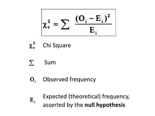
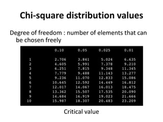
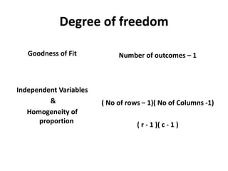
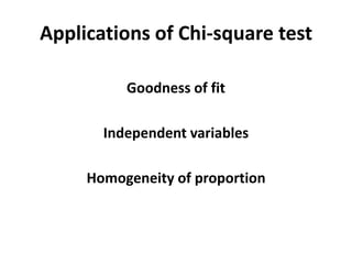
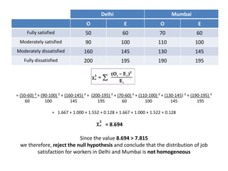
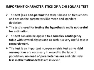
The Chi Square Test is a widely used non-parametric test that does not rely on assumptions about population parameters. It compares observed frequencies to expected frequencies specified by the null hypothesis. The Chi Square value is calculated by summing the squared differences between observed and expected values divided by the expected values. The Chi Square value is then compared to a critical value based on the degrees of freedom. Common applications include tests of goodness of fit, independence of variables, and homogeneity of proportions.

1. Chi Square Test
RAHUL BABAR

2. Chi Square Test
Simplest & the most widely used
non-parametric test in statistical work

3. NON PARAMETRIC TEST
The test don’t rely on assumptions about
population parameters:
Population Mean
Population Standard Deviation

4. Chi Square
Sum
Observed frequency
Expected (theoretical) frequency,
asserted by the null hypothesis

5. Null Hypothesis
There is no significant difference between the
observed and expected frequencies

6. Chi-square distribution values
Degree of freedom : number of elements that can
be chosen freely
Critical value

7. Degree of freedom
Goodness of Fit
Independent Variables
&
Homogeneity of
proportion
Number of outcomes – 1
( No of rows – 1)( No of Columns -1)
( r - 1 )( c - 1 )

8. Applications of Chi-square test
Goodness of fit
Independent variables
Homogeneity of proportion

9. Goodness of fit
Test of the consistency between a hypothetical
and a sample distribution.
Example : Coin is tossed 50 times
Null hypothesis is that it’s
25 times heads and 25 times tails
( expected observation E )

10. Event Frequency
Head 28
Tail 22
Total 50
Observed Values is,
Event O E O - E ( O – E ) ² ( O – E ) ²
E
Head 28 25 3 9 0.36
Tail 22 25 -3 9 0.36
Total 0.72
Solution :
= 0.72 Degree of freedom is = (outcomes – 1) = 2 – 1 = 1
Critical value is 3.841 for df 1 at 0.05
Since 0.72 < 3.841 , our null hypothesis is acceptable which means our coin is fair

11. Test of Independence
To ascertain whether there is any dependency
relationship between the two attributes.
Example: A company introduced new drug B to
cure malaria. It is being compared with
existing drug A. Data is shown in next slide.
We need to find whether the new drug B is
more effective in curing malaria.

12. Helped
(C1)
Harmed
(C2)
No effect
(C3)
Total
Drug A
(R1)
44 10 26 80
Drug B
(R2)
52 10 18 80
Total 96 20 44 160
Solution :
O E O - E ( O-E ) ² ( O – E ) ²
E
R1C1 44 48 -4 16 0.333
R1C2 10 10 0 0 0
R1C3 26 22 4 16 0.727
R2C1 52 48 4 16 0.333
R2C2 10 10 0 0 0
R2C3 18 22 -4 16 0.727
Total = 2.12

13. We setup two hypothesis,
H0 :There is no difference in the effectiveness of
the two drugs
H1 : There is difference in the effectiveness of
the two drugs
Degree of freedom = (r-1)(c-1) = (2-1)(3-1) = 2
Critical value at 0.05 for df 2 is 5.991,
and 2.12 < 5.991
So, there is no difference in the effectiveness of
the two drugs

14. Alternative method:
Helped Harmed No effect Total
Drug A 44
(a)
10
(b)
26
(c)
80
(a+b+c)
Drug B 52
(d)
10
(e)
18
(f)
80
(d+e+f)
Total 96
(a+d)
20
(b+e)
44
(c+f)
160
(N)
Its 2x3 table so for calculating chi-square we use formula:
= N a² + b² + c² + N d² + e² + f² - N
a+b+c a+d b+e c+f d+e+f a+d b+e c+f
= 160 44² + 10² + 26² + 160 52² + 10² + 18² - 160
80 96 20 44 80 96 20 44
= 2.12
Both methods give same value for which is 2.12

15. Test of homogeneity
Test indicates whether the proportions of
elements belonging to different groups in two
or more populations are similar or not.
Example : A company has two factories in Delhi
and Mumbai. It is interested to know whether
its workers are satisfied with their jobs or not
at both places.

16. Delhi Mumbai Total
Fully satisfied 50 70 120
Moderately satisfied 90 110 200
Moderately dissatisfied 160 130 290
Fully dissatisfied 200 190 390
Total 500 500 1000
We setup two hypothesis,
H0 :The proportions of workers who belong to the four job satisfaction categories are
the same in both Delhi and Mumbai
H1 : The proportions of workers who belong to the four job satisfaction categories are
not the same in both Delhi and Mumbai
Degrees of freedom = (r-1)(c-1) = (4-1)(2-1) = 3
Critical value for 3 df at 0.05 is 7.815

17. Delhi Mumbai
O E O E
Fully satisfied 50 60 70 60
Moderately satisfied 90 100 110 100
Moderately dissatisfied 160 145 130 145
Fully dissatisfied 200 195 190 195
= (50-60) ² + (90-100) ² + (160-145) ² + (200-195) ² + (70-60) ² + (110-100) ² + (130-145) ² + (190-195) ²
60 100 145 195 60 100 145 195
= 1.667 + 1.000 + 1.552 + 0.128 + 1.667 + 1.000 + 1.522 + 0.128
= 8.694
Since the value 8.694 > 7.815
we therefore, reject the null hypothesis and conclude that the distribution of job
satisfaction for workers in Delhi and Mumbai is not homogeneous

18. IMPORTANT CHARACTERISTICS OF A CHI SQUARE TEST
 This test (as a non-parametric test) is based on frequencies
and not on the parameters like mean and standard
deviation.
 The test is used for testing the hypothesis and is not useful
for estimation.
 This test can also be applied to a complex contingency
table with several classes and as such is a very useful test in
research work.
 This test is an important non-parametric test as no rigid
assumptions are necessary in regard to the type of
population, no need of parameter values and relatively
less mathematical details are involved.