The document outlines various chi-square tests, including the goodness of fit test, test for independence, and test for variance, detailing their purposes and methodologies. It provides examples to illustrate how to apply these tests, including hypothesis formulation and statistical conclusions based on p-values. The results of specific case studies reinforce the application of these concepts, demonstrating significant differences in observed versus expected frequencies in different scenarios.

1. CHI-SQUARE TESTS

2. Chi- Square Statistic
If X~𝑁(𝜇, 𝜎2) then 𝑍 =
𝑋−𝜇
𝜎
~𝑁(0,1) and
𝑍2
=
𝑋−𝜇
𝜎
2
~𝜒2
with 1 d.f. and
𝑋−𝜇
𝜎
2
~𝜒2
with n d.f.

3. Chi- Square
test
There are three types of chi-square tests.
• A Chi-square goodness of fit test determines if distribution of
sample data matches with the distribution of population.
• A Chi-square test for independence is to test whether two
categorical variables differ from each another.
• A Chi-square test for variance of single sample is to test
whether there is significant difference between sample variance
and population variance

4. Chi- Square test
– Independence of
Attributes
Chi-Square test is a statistical method to determine if
two categorical variables have a significant
correlation/association between them.

5. To test independence of attributes
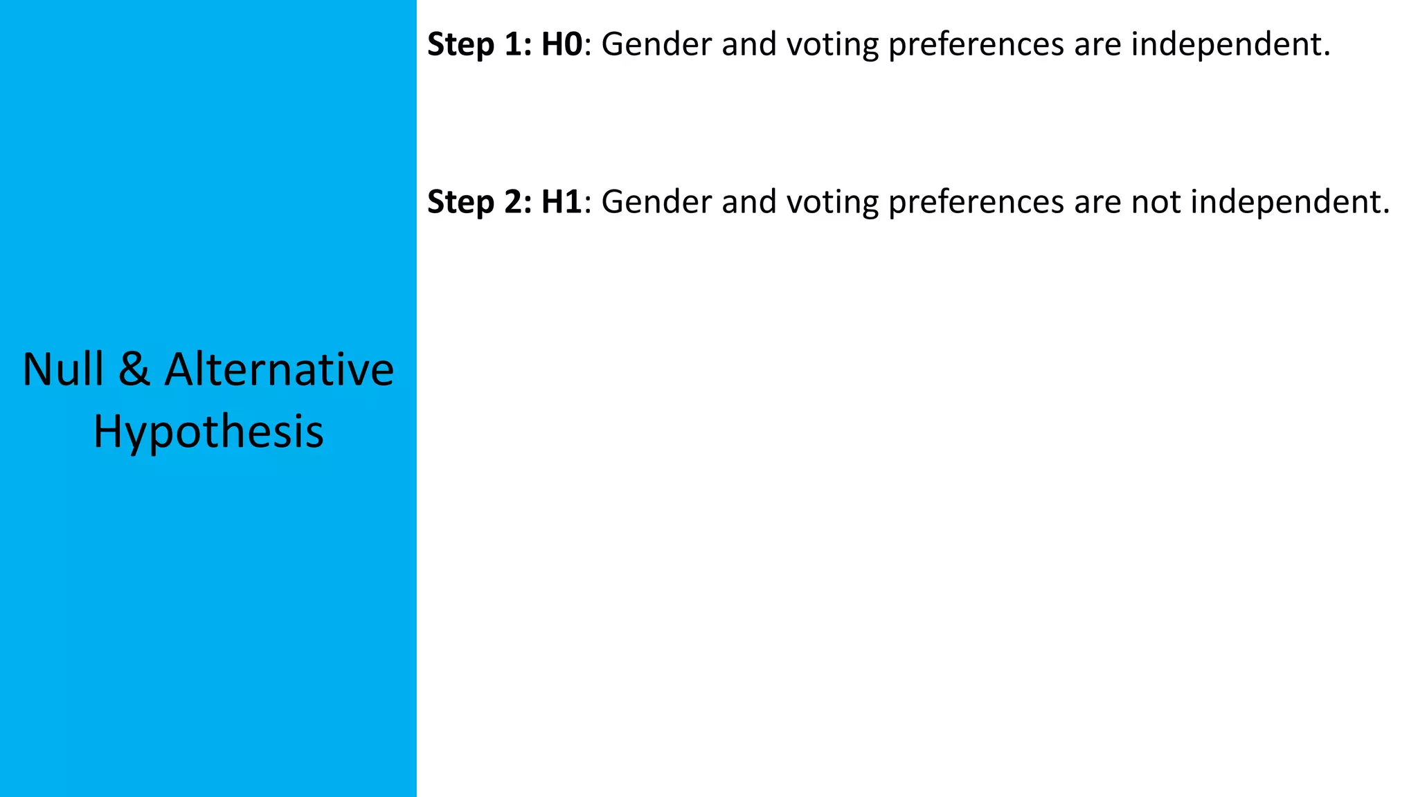
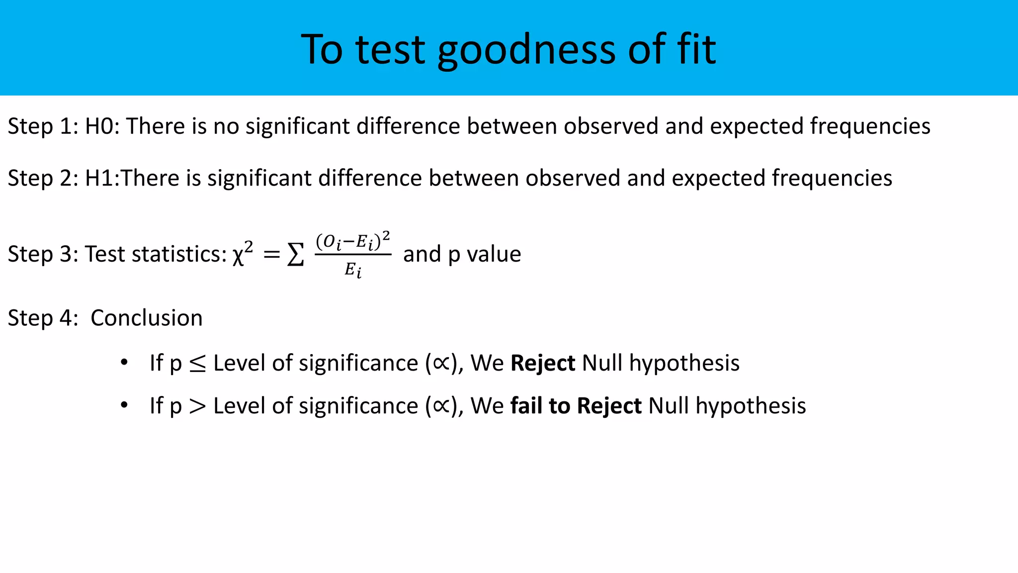
Step 1: H0: Two attributes (categorical variables) are independent
Step 2: H1: Two attributes (categorical variables) are dependent
Step 3: Test statistics: χ2 =
(𝑂𝑖−𝐸𝑖)2
𝐸𝑖
where 𝐸𝑖 =
𝑅𝑜𝑤 𝑡𝑜𝑡𝑎𝑙 ∗𝐶𝑜𝑙𝑢𝑚𝑛 𝑡𝑜𝑡𝑎𝑙
𝐺𝑟𝑎𝑛𝑑 𝑡𝑜𝑡𝑎𝑙
Step 4: Conclusion
• If p ≤ Level of significance (∝), We Reject Null hypothesis
• If p > Level of significance (∝), We fail to Reject Null hypothesis
[Note: In 2*2 contingency table if expected is less than 5, use Yate’s correction i.e. Continuity
correction in the SPSS output]

6. Example
A public opinion poll surveyed a simple random sample of 1000 voters. Respondents were
classified by gender (male or female) and by voting preference (Party A, Party B, or Party C).
Results are shown in the contingency table below. Is voting preference affected by gender?
Gender
Voting Preference
Party A Party B Party C
Male 200 150 50
Female 250 300 50

7. Null & Alternative
Hypothesis
Step 1: H0: Gender and voting preferences are independent.
Step 2: H1: Gender and voting preferences are not independent.

8. Data in SPSS
Gender
Voting Preference
Party A Party B Party C
Male 200 150 50
Female 250 300 50

9. Assigning weights

10. Chi-Square test

11. Chi-Square test

12. Chi-Square test

13. Output
The Chi-square value is 16.204 and p value = 0.000 < 0.05.
We reject the Null hypothesis.
∴ Gender and voting preferences are not independent.
i.e. voting preference is affected by gender

14. To test goodness of fit
Step 1: H0: There is no significant difference between observed and expected frequencies
Step 2: H1:There is significant difference between observed and expected frequencies
Step 3: Test statistics: χ2 =
(𝑂𝑖−𝐸𝑖)2
𝐸𝑖
and p value
Step 4: Conclusion
• If p ≤ Level of significance (∝), We Reject Null hypothesis
• If p > Level of significance (∝), We fail to Reject Null hypothesis

15. Example1
The number of road accidents on a particular highway during a week is given below. Can it be
concluded that the proportion of accidents are equal for all days?
Day Mon Tue Wed Thu Fri Sat Sun
Accidents 14 16 8 12 11 9 14

16. Hypothesis
Null Hypothesis: H0: Proportion of accidents are equal for
all days
Alternative Hypothesis: H1: Proportion of accidents are
not equal for all days

17. Day Accidents
Mon 14
Tue 16
Wed 8
Thu 12
Fri 11
Sat 9
Sun 14

18. Chi-Square test

19. Chi-Square test

20. Output
Chi-Square statistics = 4.167
p value = 0.657 > 0.05
Ho is accepted
So, it can be concluded that the proportion of
accidents are equal for all days

21. Example 2
Suppose it was suspected an unusual distribution
of blood groups in patients undergoing one type of
surgical procedure. It is known that the expected
distribution for the population served by the
hospital which performs this surgery is 44% group
O, 45% group A, 8% group B and 3% group AB. A
random sample of 187 routine pre-operative blood
grouping results are given below. Do this sample
match with the expected distribution.
Blood
Group
O A B AB
Patients 67 83 29 8
Results for 187 consecutive patients:

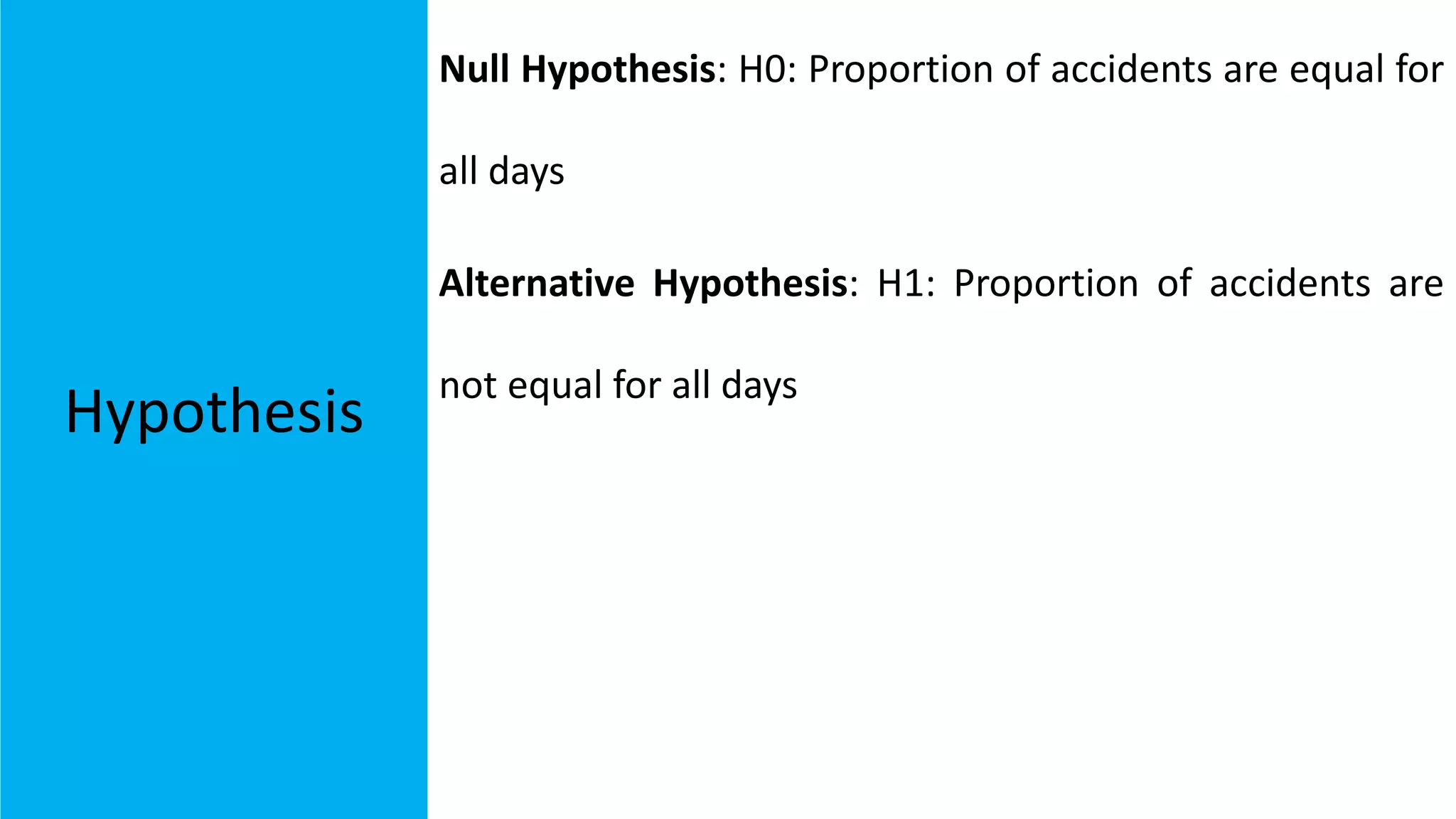
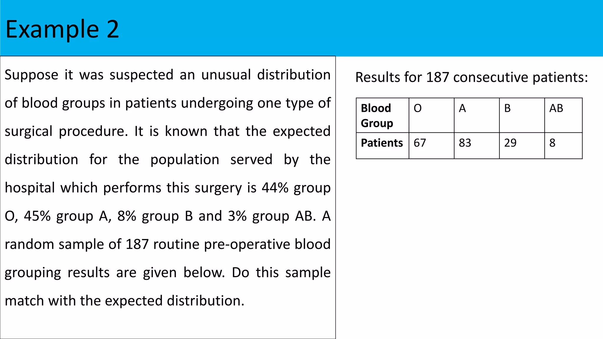
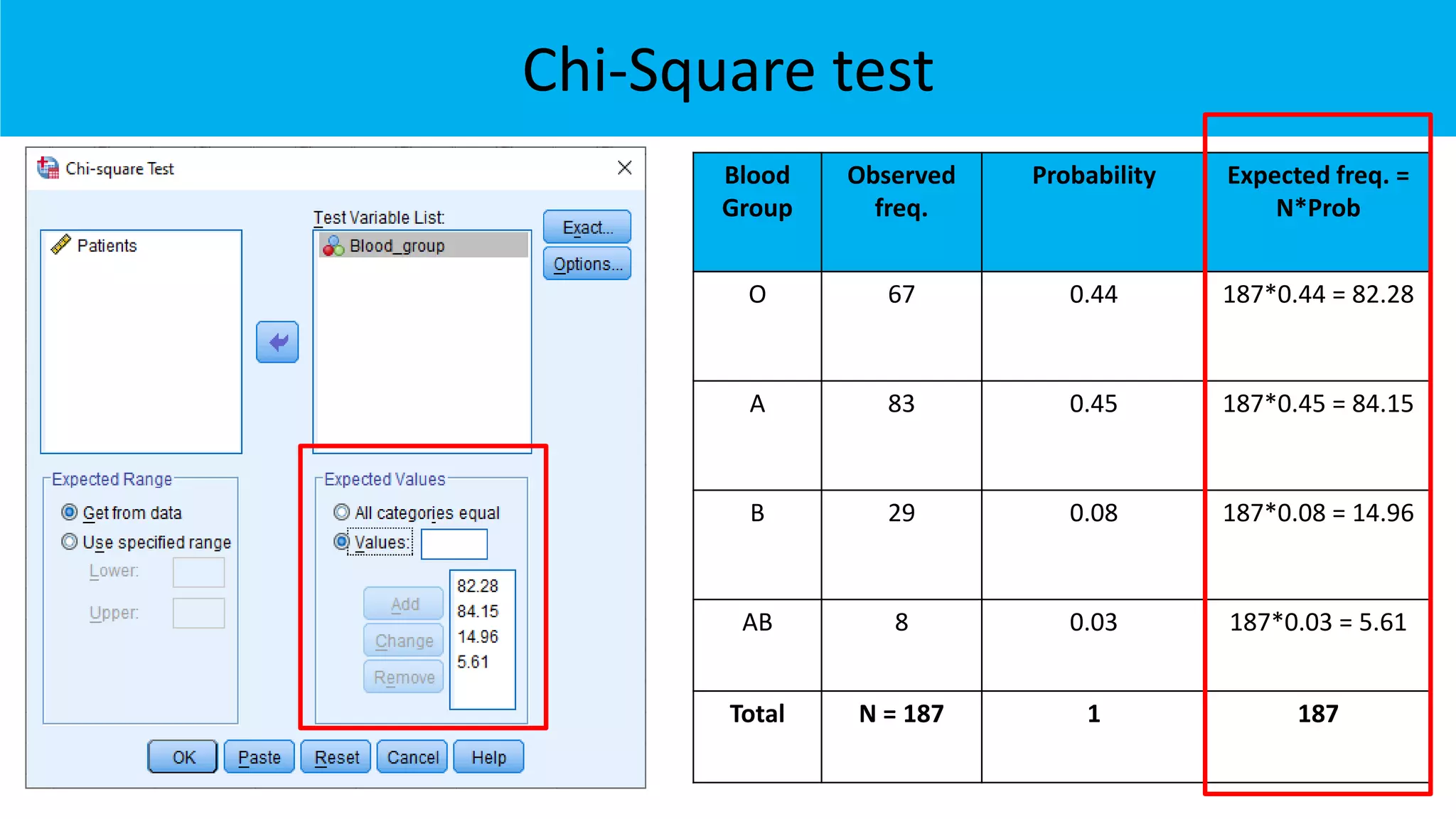
22. Hypothesis
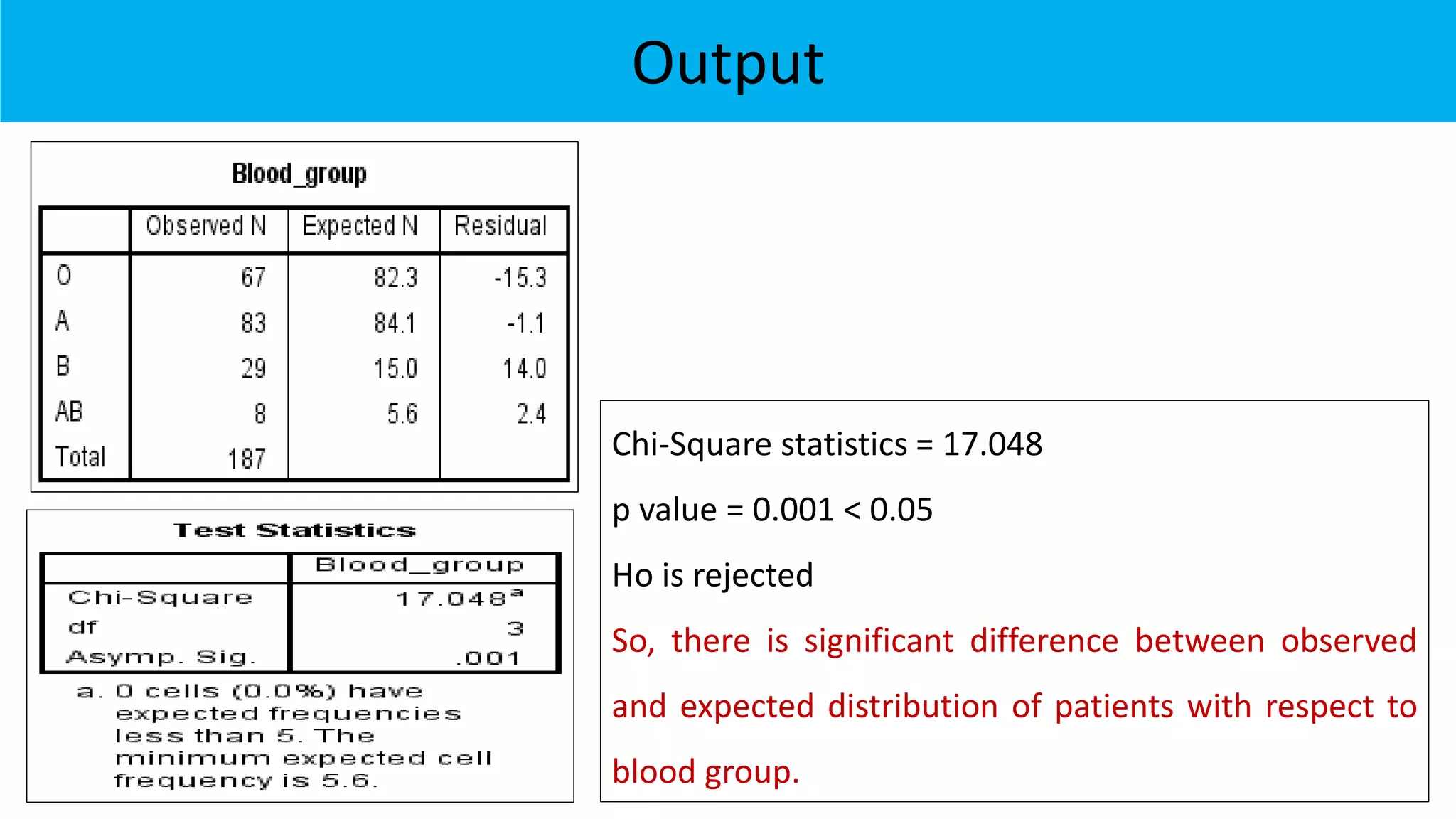
Null Hypothesis: H0: There is no significant difference
between observed and expected distribution of patients
with respect to blood group
[Sample follows expected distribution]
Alternative Hypothesis: H1: There is significant difference
between observed and expected distribution of patients
with respect to blood group
[Sample does not follows expected distribution]

23. Case Study 1
Blood
Group
Observed
freq.
O 67
A 83
B 29
AB 8
Total N = 187

24. Case Study 1
Expected distribution for the
population served by the hospital
which performs this surgery is
44% group O,
45% group A,
8% group B and
3% group AB.
Blood
Group
Observed
freq.
Probability Expected freq. =
N*Prob
O 67 0.44 187*0.44 = 82.28
A 83 0.45 187*0.45 = 84.15
B 29 0.08 187*0.08 = 14.96
AB 8 0.03 187*0.03 = 5.61
Total N = 187 1 187

25. Chi-Square test

26. Chi-Square test

27. Chi-Square test
Blood
Group
Observed
freq.
Probability Expected freq. =
N*Prob
O 67 0.44 187*0.44 = 82.28
A 83 0.45 187*0.45 = 84.15
B 29 0.08 187*0.08 = 14.96
AB 8 0.03 187*0.03 = 5.61
Total N = 187 1 187

28. Output
Chi-Square statistics = 17.048
p value = 0.001 < 0.05
Ho is rejected
So, there is significant difference between observed
and expected distribution of patients with respect to
blood group.

29. THANK YOU
Dr Parag Shah | M.Sc., M.Phil., Ph.D. ( Statistics)
pbshah@hlcollege.edu
www.paragstatistics.wordpress.com