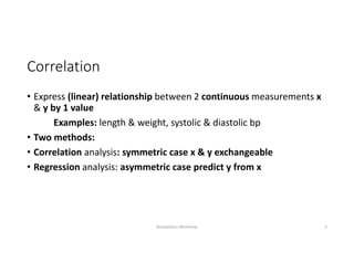
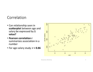
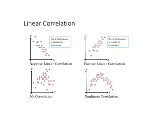
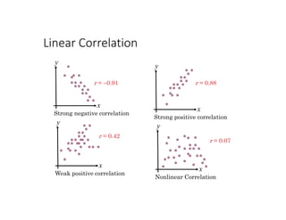
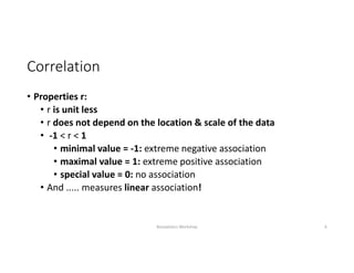
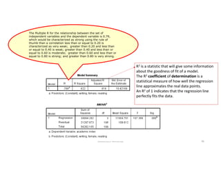
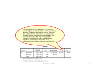
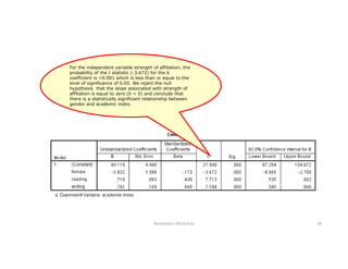
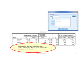
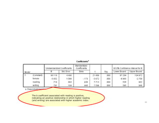
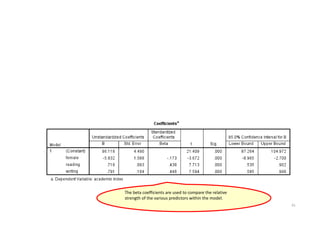
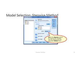
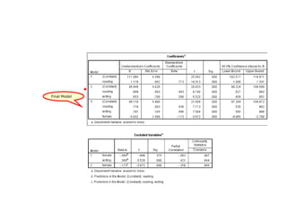
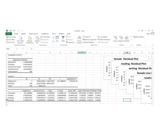
Correlation and Regression
Application with SPSS and 
Microsoft Excel
Setia Pramana
Biostatistics Workshop 1
Correlation
• Express (linear) relationship between 2 continuous measurements x 
& y by 1 value
Examples: length & weight, systolic & diastolic bp
• Two methods:
• Correlation analysis: symmetric case x & y exchangeable 
• Regression analysis: asymmetric case predict y from x
Biostatistics Workshop 2
Correlation
• Can relationship seen in 
scatterplot between age and 
salary be expressed by 1 
value?
• Pearson correlation r 
summarizes association in a 
number
• For age‐salary study: r = 0.86
Biostatistics Workshop 3
Linear Correlation
x
y
Negative Linear Correlation
x
y
No Correlation
x
y
Positive Linear Correlation
x
y
Nonlinear Correlation
As x increases,
y tends to
decrease.
As x increases,
y tends to
increase.
Linear Correlation
x
y
Strong negative correlation
x
y
Weak positive correlation
x
y
Strong positive correlation
x
y
Nonlinear Correlation
r = 0.91 r = 0.88
r = 0.42
r = 0.07
Correlation
• Properties r: 
• r is unit less
• r does not depend on the location & scale of the data
• ‐1 < r < 1
• minimal value = ‐1: extreme negative association
• maximal value = 1: extreme positive association
• special value = 0: no association
• And ..... measures linear association!
Biostatistics Workshop 6
Correlation
• Pearson correlation coefficient expresses the degree of linear relationship between 
age and salary
• Pearson correlation coefficient is useful when x & y have a Normal distribution
• When x or y has not a normal distribution, then: 
• Try transformation to Normality (log)
• Take non‐parametric technique = Spearman rank correlation
• When x and y are ordinal, then:
• Spearman rank correlation
Biostatistics Workshop 7
Correlation
• For Pearson & Spearman correlation x can be interchanged with y 
without changing the correlation. Hence correlation between age & 
salary = correlation between salary and age! 
• Pearson & Spearman correlations only measure association and not 
causation!
• Pearson & Spearman correlation coefficient are often practically 
equal, but Spearman is more robust to outliers.
Biostatistics Workshop 8
Linear Regression
• Univariate
• Multivariate (Multivariable)
Biostatistics Workshop 9
What is Linear Regression?
• The method of finding the best 
line (curve) is least squares, which 
minimizes the distance from the 
line for each of points 
• The equation of the line is y=1.5x 
+ 4
y = 1.5x + 4
0
5
10
15
20
25
0 2 4 6 8 10 12
Simple Linear Regression
• Model y = a + b x
• Simple: only 1 X
• Linear: straight line relationship 
• Terminology:x: regressor (independent variable)
• y: response (dependent variable)
• intercept, slope: regression coefficients
Biostatistics Workshop 11
Assumptions of Linear Regression
• Linearity
• Linear relationship between outcome and predictors
• E(Y|X=x)=+ x1 + 2x2
2 is still a linear regression equation 
because each of the ’s is to the first power
• Normality of the residuals
• The residuals, i, are normally distributed, N(0, 
• Homoscedasticity of the residuals
• The residuals, i, have the same variance
• Independence
• All of the data points are independent
• Correlated data points can be taken into account using 
multivariate and longitudinal data methods
• Predicting salary from Age
• Regression line
= the straight line that approximates best the data and predicts 
salary from age
is completely determined by two parameters intercept & slope
expresses the (linear) relationship of age with salary
Biostatistics Workshop 13
• The regression line for the example
salary (€) = 200.32 + 69.78 age (yrs) = regression equation
• age = 35 average salary = 2642.55 €
• age = 50 average salary = 3689.22 €
• Prediction without knowing age: Average salary = 3325.712 €
• Prediction if age is known (= 38 yrs):Average salary = 2855.521 €
Biostatistics Workshop 14
• Regression of y on x (salary on age) is not the same as the regression of x 
on y (age on salary)
Biostatistics Workshop 15
Regression: Slope
• The regression line for the example
salary (€) = 200.32 + 69.78 age (yrs) = regression equation
• age = 50 (mean) salary = 200.32 + 69.78×50
• age = 51 (mean) salary = 200.32 + 69.78×51
• Increase in age with 1 year => Increase in mean salary with 69.78 €
• Interpretation of slope = average increase in response when 
regressor increases with 1 unit
Biostatistics Workshop 16
Coefficient Determination
• Gain by knowing relation age with salary 
• improvement of prediction 
• improvement can be seen by reduction in variability
• Gain can be expressed in 1 value: R2
• R2 : percentage gain by considering regression line.
• Example:•R² = 1 ‐ 0.26 = 0.74⇒74% gain by regression model in predicting 
salary
Biostatistics Workshop 17
Multiple (Multivariate) Linear Regression
• The model is: y = b0 + b1 x1 + b2 x2 … + bp xp
= multiple linear regression model
• multiple: because of p regressors
• linear: because of straight line relationship
• Terminology:
• x1 , x2 , …,xp = regressors (independent variables)
• response (dependent variable)  y = 
• b0,b1 , b2 , …,bp = regression coefficients
Biostatistics Workshop 18
Coefficients Regression 
• There is a univariate effect of regressor/predictor on a response = 
regression coefficient in simple linear regression
= (average) increase of response when regressor increases with 1 unit
• Multiple effect of regressor on response = regression coefficient in 
multiple linear regression
= (average) increase of response when regressor increases with 1 unit 
and when other regressors are held fixed 
Biostatistics Workshop 19
Multiple (Multivariate) Linear Regression
• Study on salaries: also 100 women were included in the study
• Descriptive statistics in mean (SD):
• age men = 44.79 yrs (9.97)
• age women = 43.90 yrs (9.15)
• salary men = 3326 € (729.4)
• salary women = 2829 € (728.6)
• Now 2 regression lines, 1 for men
& 1 for women
Biostatistics Workshop 20
Multiple (Multivariate) Linear Regression
• Two regression lines (estimated separately)
• For men: salary = 200.32 + 69.78 age
• For women: salary = ‐5.97 + 64.59 age
• We see that the intercepts and the slopes are different for men & 
women. 
• What does this mean?
• Slopes differ = difference between men & women is not constant
• Intercepts differ = salary between men & women at age 0 differ?
Biostatistics Workshop 21
Multiple (Multivariate) Linear Regression
• Include dummy variable sex
• The (overall) model implies two models, one for men and one for 
women. Namely:
• For men: salary = 318.8 + 67 age
• For women: salary = 318.8 – 436.5 + 67 age
• Thus model assumes that men & women have the same slope in the 
model. 
• This means that we assume that the difference between men & 
women in mean salary is constant on average. Is this so? How can 
we test this?
Biostatistics Workshop 22
Multiple (Multivariate) Linear Regression
• To test that slopes are different for men & women:
• Enlarge model again, namely include variable age*sex which is simply the 
product of age and sex. Thus:
• age*sex = 0 for a man age*sex = age for a woman
• Fit model with age, sex & age*sex predicting salary
• salary = 2000.3 + 69.8 age –206.3 sex – 5.2 age*sex
• P‐value for regression coefficient of age*sex = 0.47
• ⇒We do believe that women earn less than men but that the difference is 
independent of age.
Biostatistics Workshop 23
SPSS
• Datasets are available at 
https://sites.google.com/site/biostatinfocore/home/regressionspss
Biostatistics Workshop 24
SPSS
• Data Input
• Data View
Biostatistics Workshop 25
• Variable View
Biostatistics Workshop 26
Scatter Plot
Biostatistics Workshop 27
Plotting
• Scatter Plot
Biostatistics Workshop 28
Plotting
• Scatter Plot
Biostatistics Workshop 29
Plotting
Scatter plot by group
Biostatistics Workshop 30
Plotting
Matrix Scatter plot
Biostatistics Workshop 31
Regression
Request a standard
Liner or multiple
regression
Biostatistics Workshop 32
Specify the 
variables and 
selection 
method
Biostatistics Workshop 33
• Output
Biostatistics Workshop 34
Biostatistics Workshop 35
Biostatistics Workshop 36
The Multiple R for the relationship between the set of
independent variables and the dependent variable is 0.79,
which would be characterized as strong using the rule of
thumb than a correlation less than or equal to 0.20 is
characterized as very weak; greater than 0.20 and less than
or equal to 0.40 is weak; greater than 0.40 and less than or
equal to 0.60 is moderate; greater than 0.60 and less than or
equal to 0.80 is strong; and greater than 0.80 is very strong.
R2 is a statistic that will give some information 
about the goodness of fit of a model. 
The R2 coefficient of determination is a 
statistical measure of how well the regression 
line approximates the real data points. 
An R2 of 1 indicates that the regression line 
perfectly fits the data.
Biostatistics Workshop 37
The probability of the F statistic (107.4) for the
overall regression relationship is <0.001, less than or
equal to the level of significance of 0.05. We reject
the null hypothesis that there is no relationship
between the set of independent variables and the
dependent variable (R² = 0). We support the
research hypothesis that there is a statistically
significant relationship between the set of
independent variables and the dependent variable.
Biostatistics Workshop 38
For the independent variable strength of affiliation, the
probability of the t statistic (-3.672) for the b
coefficient is <0.001 which is less than or equal to the
level of significance of 0.05. We reject the null
hypothesis that the slope associated with strength of
affiliation is equal to zero (b = 0) and conclude that
there is a statistically significant relationship between
gender and academic index.
Biostatistics Workshop 39
The b coefficient associated with gender (-5.8) is
negative, indicating that Male has lower academic index
as compared female student.
Biostatistics Workshop 40
The b coefficient associated with reading is positive,
indicating an positive relationship in which higher reading
(and writing) are associated with higher academic index.
Biostatistics Workshop 41
The beta coefficients are used to compare the relative 
strength of the various predictors within the model.
Model Selection: Stepwise Method
Biostatistics Workshop 42
Select the Stepwise method
for entering the variables
into the analysis from the
drop down Method menu.
Biostatistics Workshop 43
Final Model
Regression using Ms. Excel
Biostatistics Workshop 44
Correlation & Regression using Ms. Excel
Biostatistics Workshop 45
Biostatistics Workshop 46
Biostatistics Workshop 47
Biostatistics Workshop 48
Now try with different datasets!
Biostatistics Workshop 49

Correlation and Regression Analysis using SPSS and Microsoft Excel