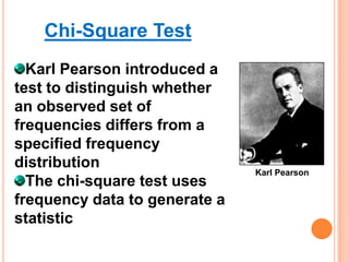
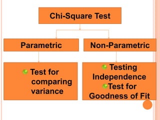
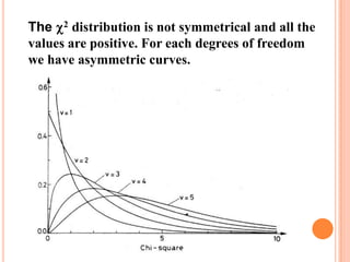
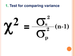
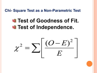
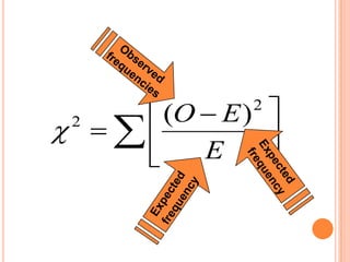
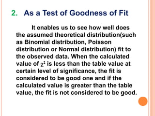
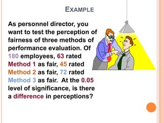
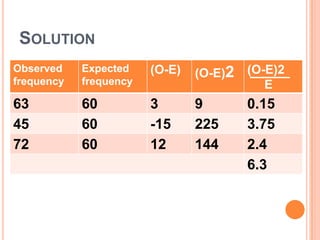
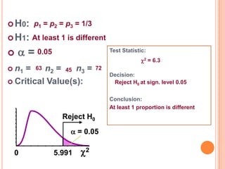
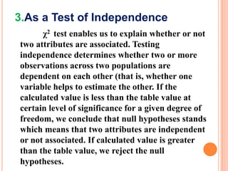
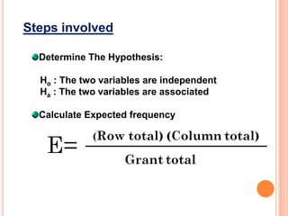
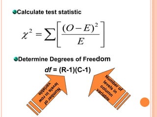
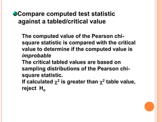
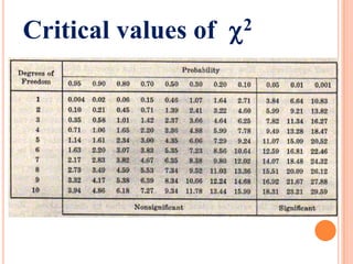
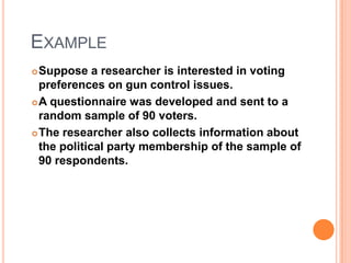
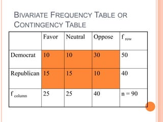
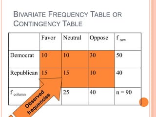
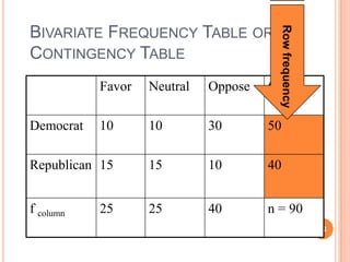
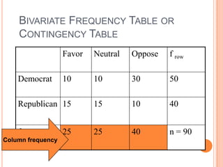
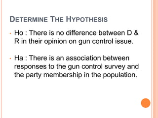
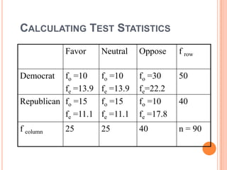
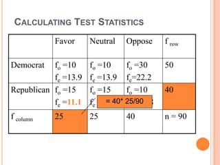
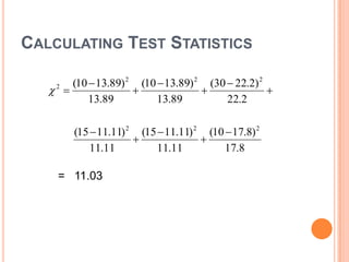
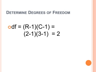
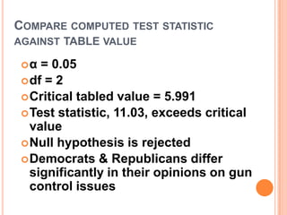
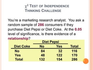
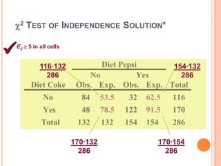
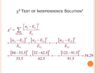
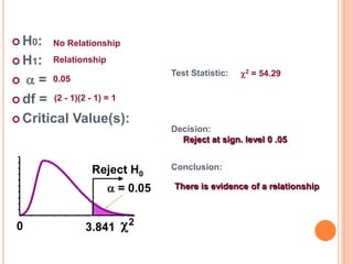
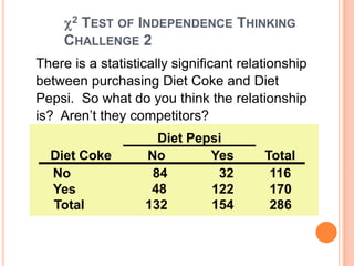
The document discusses the chi-square test, which is used to determine if an observed frequency distribution differs from an expected theoretical distribution. It can be used as a test of independence to determine if two variables are associated, and as a test of goodness of fit to assess how well an expected distribution fits observed data. The steps of the chi-square test are outlined, including calculating the test statistic, determining degrees of freedom, and comparing the statistic to critical values to determine if the null hypothesis can be rejected. An example of a chi-square test of independence is shown to test if perceptions of fairness of performance evaluation methods are independent of each other.

1. Anandapadmanabhan J.
S1 M.Com

2. Chi-Square Test
Karl Pearson introduced a
test to distinguish whether
an observed set of
frequencies differs from a
specified frequency
distribution
The chi-square test uses
frequency data to generate a
statistic
Karl Pearson

3. A chi-square test is a statistical test
commonly used for testing independence
and goodness of fit. Testing independence
determines whether two or more
observations across two populations are
dependent on each other (that is, whether
one variable helps to estimate the other).
Testing for goodness of fit determines if
an observed frequency distribution
matches a theoretical frequency
distribution.

4. Chi-Square Test
Parametric
Test for
comparing
variance
Non-Parametric
Testing
Independence
Test for
Goodness of Fit

5. Conditions for the application of 2 test
Observations recorded and collected are
collected on random basis.
All items in the sample must be
independent.
No group should contain very few items,
say less than 10. Some statisticians take this
number as 5. But 10 is regarded as better by
most statisticians.
Total number of items should be large, say
at least 50.

6. The 2 distribution is not symmetrical and all the
values are positive. For each degrees of freedom
we have asymmetric curves.

7. 1. Test for comparing variance
2 =


8. Chi- Square Test as a Non-Parametric Test
Test of Goodness of Fit.
Test of Independence.
 (O  E ) 
2
  

E


2

9.  (O  E ) 
2
  

E


2

10. 2. As a Test of Goodness of Fit
It enables us to see how well does
the assumed theoretical distribution(such
as Binomial distribution, Poisson
distribution or Normal distribution) fit to
the observed data. When the calculated
value of χ2 is less than the table value at
certain level of significance, the fit is
considered to be good one and if the
calculated value is greater than the table
value, the fit is not considered to be good.

11. EXAMPLE
As personnel director, you
want to test the perception of
fairness of three methods of
performance evaluation. Of
180 employees, 63 rated
Method 1 as fair, 45 rated
Method 2 as fair, 72 rated
Method 3 as fair. At the 0.05
level of significance, is there
a difference in perceptions?

12. SOLUTION
Observed
frequency
Expected
frequency
(O-E)
(O-E)2
(O-E)2
E
63
45
72
60
60
60
3
-15
12
9
225
144
0.15
3.75
2.4
6.3

13.  H0: p1 = p2 = p3 = 1/3
 H1: At least 1 is different

 = 0.05
Test Statistic:
2 = 6.3
 n1
= 63 n2 = 45 n3 =
 Critical Value(s):
72
Decision:
Reject H0 at sign. level 0.05
Conclusion:
At least 1 proportion is different
Reject H0
 = 0.05
0
5.991
2

14. 3.As a Test of Independence
χ2 test enables us to explain whether or not
two attributes are associated. Testing
independence determines whether two or more
observations across two populations are
dependent on each other (that is, whether one
variable helps to estimate the other. If the
calculated value is less than the table value at
certain level of significance for a given degree of
freedom, we conclude that null hypotheses stands
which means that two attributes are independent
or not associated. If calculated value is greater
than the table value, we reject the null
hypotheses.

15. Steps involved
Determine The Hypothesis:
Ho : The two variables are independent
Ha : The two variables are associated
Calculate Expected frequency

16. Calculate test statistic
 (O  E ) 
  

E


2
2
Determine Degrees of Freedom
df = (R-1)(C-1)

17. Compare computed test statistic
against a tabled/critical value
The computed value of the Pearson chisquare statistic is compared with the critical
value to determine if the computed value is
improbable
The critical tabled values are based on
sampling distributions of the Pearson chisquare statistic.
If calculated 2 is greater than 2 table value,
reject Ho

18. Critical values of
2


19. EXAMPLE
Suppose a researcher is interested in voting
preferences on gun control issues.
 A questionnaire was developed and sent to a
random sample of 90 voters.
 The researcher also collects information about
the political party membership of the sample of
90 respondents.


20. BIVARIATE FREQUENCY TABLE OR
CONTINGENCY TABLE
Favor
Neutral
Oppose
f row
10
10
30
50
Republican 15
15
10
40
f column
25
40
n = 90
Democrat
25

21. BIVARIATE FREQUENCY TABLE OR
CONTINGENCY TABLE
Favor
Neutral
Oppose
f row
10
10
30
50
Republican 15
15
10
40
f column
25
40
n = 90
Democrat
25

22. Row frequency
BIVARIATE FREQUENCY TABLE OR
CONTINGENCY TABLE
Favor
Neutral
Oppose
f row
10
10
30
50
Republican 15
15
10
40
f column
25
40
n = 90
Democrat
25
22

23. BIVARIATE FREQUENCY TABLE OR
CONTINGENCY TABLE
Favor
Neutral
Oppose
f row
10
10
30
50
Republican 15
15
10
40
f column
25
40
n = 90
Democrat
Column frequency
25

24. DETERMINE THE HYPOTHESIS
•
Ho : There is no difference between D &
R in their opinion on gun control issue.
•
Ha : There is an association between
responses to the gun control survey and
the party membership in the population.

25. CALCULATING TEST STATISTICS
Favor
Neutral
Oppose
f row
fo =10
fe =13.9
Republican fo =15
fe =11.1
fo =10
fe =13.9
fo =15
fe =11.1
fo =30
fe=22.2
fo =10
fe =17.8
50
f column
25
40
n = 90
Democrat
25
40

26. CALCULATING TEST STATISTICS
Favor
Democrat
Neutral
Oppose
f row
fo =10
fe =13.9
Republican fo =15
fe =11.1
fo =10
fo =30
fe =13.9 fe=22.2
fo =15
fo =10
= 40* fe =17.8
fe =11.1 25/90
50
f column
25
n = 90
25
40
40

27. CALCULATING TEST STATISTICS
(10  13.89) 2 (10  13.89) 2 (30  22.2) 2
 



13.89
13.89
22.2
2
(15  11.11) 2 (15  11.11) 2 (10  17.8) 2


11.11
11.11
17.8
= 11.03

28. DETERMINE DEGREES OF FREEDOM
df
= (R-1)(C-1) =
(2-1)(3-1) = 2

29. COMPARE COMPUTED TEST STATISTIC
AGAINST TABLE VALUE
α
= 0.05
 df = 2
 Critical tabled value = 5.991
 Test statistic, 11.03, exceeds critical
value
 Null hypothesis is rejected
 Democrats & Republicans differ
significantly in their opinions on gun
control issues

30. 2 TEST OF INDEPENDENCE
THINKING CHALLENGE
You’re a marketing research analyst. You ask a
random sample of 286 consumers if they
purchase Diet Pepsi or Diet Coke. At the 0.05
level of significance, is there evidence of a
relationship?
Diet Pepsi
Diet Coke
No
Yes
Total
No
84
32
116
Yes
48
122
170
Total
132
154
286

31. 2 TEST OF INDEPENDENCE SOLUTION*

Eij  5 in all cells
116·132
286
Diet Coke
Diet Pepsi
154·132
286
No
Yes
Obs. Exp. Obs. Exp. Total
No
84
53.5
32
62.5
116
Yes
48
78.5
122
91.5
170
Total
132
132
154
154
286
170·132
286
170·154
286

32. 2 TEST OF INDEPENDENCE SOLUTION*
 nij  Eij 


  
Eij
all cells
2
2
 n11  E11 

 n12  E12 

2
2
E11
E12
84  53.5

2
53.5
 n22  E22 
 
2
E22
32  62.5

2
62.5
122  91.5
 
2
91.5
 54.29

33.  H0:
No Relationship
 H1:
Relationship
 = 0.05
 df = (2 - 1)(2 - 1) = 1
 Critical Value(s):

Test Statistic:
2 = 54.29
Decision:
Reject at sign. level 0 .05
Reject H0
 = 0.05
0
3.841
2
Conclusion:
There is evidence of a relationship

34. 2 TEST OF INDEPENDENCE THINKING
CHALLENGE 2
There is a statistically significant relationship
between purchasing Diet Coke and Diet
Pepsi. So what do you think the relationship
is? Aren’t they competitors?
Diet Coke
No
Yes
Total
Diet Pepsi
No
Yes
84
32
48
122
132
154
Total
116
170
286

35. YOU RE-ANALYZE THE DATA
High
Income
Diet Coke
No
Yes
Total
Diet Pepsi
No
Yes
4
30
40
2
44
32
Total
34
42
76
Diet Coke
No
Yes
Total
Diet Pepsi
No
Yes
80
2
8
120
88
122
Total
82
128
210
Low
Income
Data mining example: no need for statistics here!

36. TRUE RELATIONSHIPS*
Diet Coke
Underlying
causal relation
Control or
intervening variable
(true cause)
Apparent
relation
Diet Pepsi

37. MORAL OF THE STORY
Numbers don’t
think - People
do!

38. CONCLUSION
1.
Explained 2 Test for Proportions
2.
Explained 2 Test of Independence