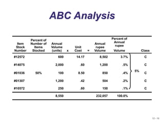
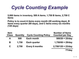
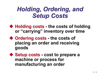
The document discusses inventory management. It defines the objective of inventory management as balancing inventory investment and customer service. There are different types of inventory like raw materials, work-in-process, and finished goods. Effective inventory management requires classifying inventory items and maintaining accurate records. The ABC analysis method divides inventory into classes based on annual dollar usage to focus management on critical items. The economic order quantity (EOQ) model can determine the optimal order quantity to minimize total inventory costs considering setup and holding costs. The reorder point indicates when to place a new order based on lead time and daily demand.


![12 - 43
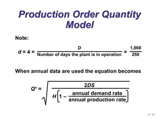
Production Order Quantity
Model
Q = Number of pieces per order p = Daily production rate
H = Holding cost per unit per year d = Daily demand/usage rate
D = Annual demand
Q2 =
2DS
H[1 - (d/p)]
Q* =
2DS
H[1 - (d/p)]
p
Setup cost = (D/Q)S
Holding cost = HQ[1 - (d/p)]
1
2
(D/Q)S = HQ[1 - (d/p)]
1
2](https://image.slidesharecdn.com/5a-inventorymgt-220920092325-613ce4be/85/5A-INVENTORY-MGT-ppt-43-320.jpg)
![12 - 44
Production Order Quantity
Example
D = 1,000 units p = 8 units per day
S = $10 d = 4 units per day
H = $0.50 per unit per year
Q* =
2DS
H[1 - (d/p)]
= 282.8 or 283 hubcaps
Q* = = 80,000
2(1,000)(10)
0.50[1 - (4/8)]](https://image.slidesharecdn.com/5a-inventorymgt-220920092325-613ce4be/85/5A-INVENTORY-MGT-ppt-44-320.jpg)