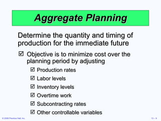
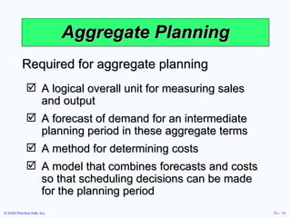
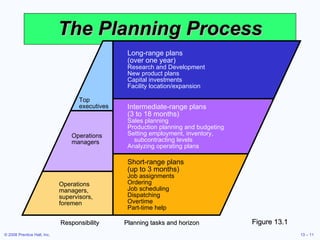
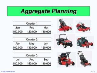
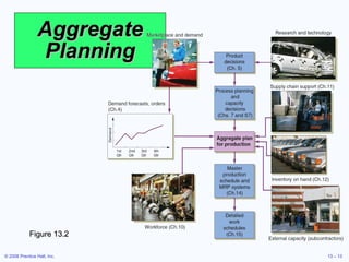
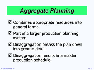
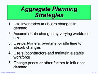
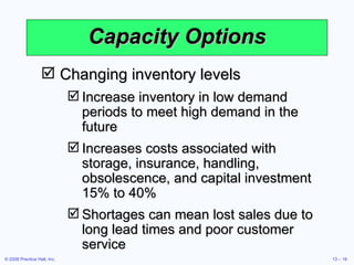
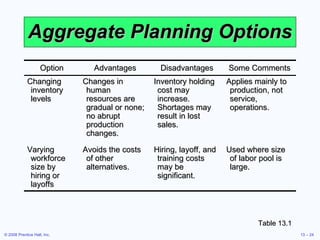
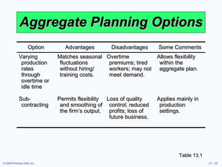
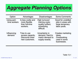
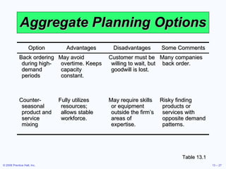
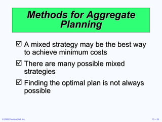
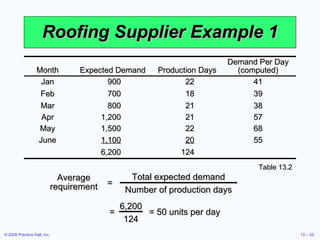
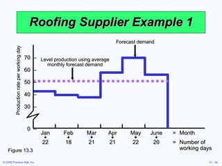
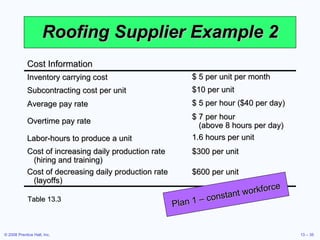
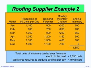
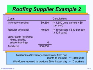
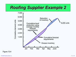
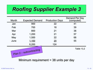
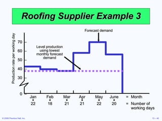
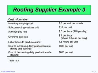
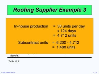
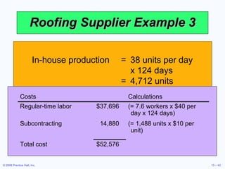
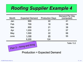
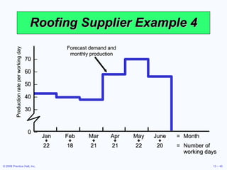
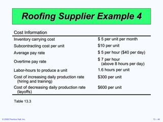
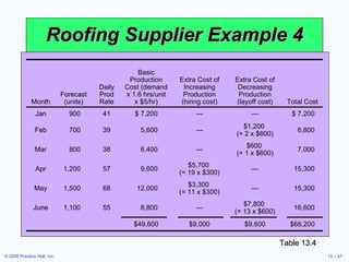
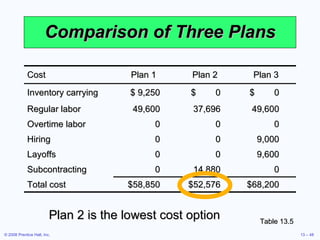
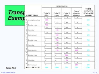
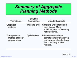
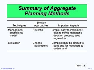
Operations Management Session 4 –  Aggregate Planning
Outline Global Company Profile:  Anheuser-Busch The Planning Process The Nature of Aggregate Planning Aggregate Planning Strategies Capacity Options Demand Options Mixing Options to Develop a Plan
Outline – Continued Methods for Aggregate Planning Graphical Methods Mathematical Approaches Comparison of Aggregate Planning Methods
Outline – Continued Aggregate Planning in Services Restaurants Hospitals National Chains of Small Service Firms Miscellaneous Services   Airline Industry Yield Management
Learning Objectives When you complete this chapter you should be able to: Define aggregate planning Identify optional strategies for developing an aggregate plan Prepare a graphical aggregate plan
Learning Objectives When you complete this chapter you should be able to: Solve an aggregate plan via the transportation method of linear programming Understand and solve a yield management problem
Anheuser-Busch Anheuser-Busch produces nearly 40% of the beer consumed in the U.S. Matches fluctuating demand by brand to plant, labor, and inventory capacity to achieve high facility utilization High facility utilization requires Meticulous cleaning between batches Effective maintenance Efficient employee and facility scheduling
Anheuser-Busch Product-focused facility with high fixed costs High utilization requires effective aggregate planning of the four basic stages of production Selection and delivery of raw materials Brewing process from milling to aging Packaging Distribution
Aggregate Planning Objective is to minimize cost over the planning period by adjusting Production rates Labor levels Inventory levels Overtime work Subcontracting rates Other controllable variables Determine the quantity and timing of production for the immediate future
Aggregate Planning A logical overall unit for measuring sales and output A forecast of demand for an intermediate planning period in these aggregate terms A method for determining costs A model that combines forecasts and costs so that scheduling decisions can be made for the planning period Required for aggregate planning
The Planning Process Figure 13.1 Long-range plans  (over one year) Research and Development New product plans Capital investments Facility location/expansion Intermediate-range plans  (3 to 18 months) Sales planning Production planning and budgeting Setting employment, inventory, subcontracting levels Analyzing operating plans Short-range plans  (up to 3 months) Job assignments Ordering Job scheduling Dispatching Overtime Part-time help Top executives Operations managers Operations managers, supervisors, foremen Responsibility Planning tasks and horizon
Aggregate Planning Quarter 1 Jan Feb Mar 150,000 120,000 110,000 Quarter 2 Apr May Jun 100,000 130,000 150,000 Quarter 3 Jul Aug Sep 180,000 150,000 140,000
Aggregate Planning Figure 13.2
Aggregate Planning Combines appropriate resources into general terms Part of a larger production planning system Disaggregation breaks the plan down into greater detail Disaggregation results in a master production schedule
Aggregate Planning Strategies Use inventories to absorb changes in demand Accommodate changes by varying workforce size Use part-timers, overtime, or idle time to absorb changes Use subcontractors and maintain a stable workforce Change prices or other factors to influence demand
Capacity Options Changing inventory levels Increase inventory in low demand periods to meet high demand in the future Increases costs associated with storage, insurance, handling, obsolescence, and capital investment 15% to 40% Shortages can mean lost sales due to long lead times and poor customer service
Capacity Options Varying workforce size by hiring or layoffs Match production rate to demand Training and separation costs for hiring and laying off workers  New workers may have lower productivity Laying off workers may lower morale and productivity
Capacity Options Varying production rate through overtime or idle time Allows constant workforce May be difficult to meet large increases in demand Overtime can be costly and may drive down productivity Absorbing idle time may be difficult
Capacity Options Subcontracting Temporary measure during periods of peak demand May be costly Assuring quality and timely delivery may be difficult Exposes your customers to a possible competitor
Capacity Options Using part-time workers Useful for filling unskilled or low skilled positions, especially in services
Demand Options Influencing demand Use advertising or promotion to increase demand in low periods Attempt to shift  demand to slow  periods May not be  sufficient to  balance demand  and capacity
Demand Options Back ordering during high- demand periods Requires customers to wait for an order without loss of goodwill or the order Most effective when there are few if any substitutes for the product or service Often results in lost sales
Demand Options Counterseasonal product and service mixing Develop a product mix of counterseasonal items May lead to products or services outside the company’s areas of expertise
Aggregate Planning Options Table 13.1 Option Advantages Disadvantages Some Comments Changing inventory levels Changes in human resources are gradual or none; no abrupt production changes. Inventory holding cost may increase. Shortages may result in lost sales. Applies mainly to production, not service, operations. Varying workforce size by hiring or layoffs Avoids the costs of other alternatives. Hiring, layoff, and training costs may be significant. Used where size of labor pool is large.
Aggregate Planning Options Table 13.1 Option Advantages Disadvantages Some Comments Varying production rates through overtime or idle time Matches seasonal fluctuations without hiring/ training costs. Overtime premiums; tired workers; may not meet demand. Allows flexibility within the aggregate plan. Sub-contracting Permits flexibility and smoothing of the firm’s output. Loss of quality control; reduced profits; loss of future business. Applies mainly in production settings.
Aggregate Planning Options Table 13.1 Option Advantages Disadvantages Some Comments Using part-time workers Is less costly and more flexible than full-time workers. High turnover/ training costs; quality suffers; scheduling difficult. Good for unskilled jobs in areas with large temporary labor pools. Influencing demand Tries to use excess capacity. Discounts draw new customers. Uncertainty in demand. Hard to match demand to supply exactly. Creates marketing ideas. Overbooking used in some businesses.
Aggregate Planning Options Table 13.1 Option Advantages Disadvantages Some Comments Back ordering during high-demand periods May avoid overtime. Keeps capacity constant. Customer must be willing to wait, but goodwill is lost. Many companies back order. Counter-seasonal product and service mixing Fully utilizes resources; allows stable workforce. May require skills or equipment outside the firm’s areas of expertise. Risky finding products or services with opposite demand patterns.
Methods for Aggregate Planning A mixed strategy may be the best way to achieve minimum costs There are many possible mixed strategies Finding the optimal plan is not always possible
Mixing Options to  Develop a Plan Chase strategy Match output rates to demand forecast for each period Vary workforce levels or vary production rate Favored by many service organizations
Mixing Options to  Develop a Plan Level strategy Daily production is uniform Use inventory or idle time as buffer Stable production leads to better quality and productivity Some combination of capacity options, a mixed strategy, might be the best solution
Graphical Methods Popular techniques Easy to understand and use Trial-and-error approaches that do not guarantee an optimal solution Require only limited computations
Graphical Methods Determine the demand for each period Determine the capacity for regular time, overtime, and subcontracting each period Find labor costs, hiring and layoff costs, and inventory holding costs Consider company policy on workers and stock levels Develop alternative plans and examine their total costs
Roofing Supplier Example 1 Table 13.2 Month Expected Demand Production Days Demand Per Day (computed) Jan 900 22 41 Feb 700 18 39 Mar 800 21 38 Apr 1,200 21 57 May 1,500 22 68 June 1,100   20 55 6,200 124 =  = 50 units per day 6,200 124 Average requirement = Total expected demand Number of production days
Roofing Supplier Example 1 Figure 13.3 70  – 60  – 50  – 40  – 30  – 0  – Jan Feb Mar Apr May June = Month       22 18 21 21 22 20 = Number of working days Production rate per working day Level production using average monthly forecast demand Forecast demand
Roofing Supplier Example 2 Table 13.3 Plan 1 – constant workforce Cost Information Inventory carrying cost $ 5 per unit per month Subcontracting cost per unit $10 per unit Average pay rate $ 5 per hour ($40 per day) Overtime pay rate $ 7 per hour  (above 8 hours per day) Labor-hours to produce a unit 1.6 hours per unit Cost of increasing daily production rate (hiring and training) $300 per unit Cost of decreasing daily production rate (layoffs) $600 per unit
Roofing Supplier Example 2 Table 13.3 Plan 1 – constant workforce Total units of inventory carried over from one month to the next = 1,850 units Workforce required to produce 50 units per day = 10 workers Cost Information Inventory carry cost $ 5 per unit per month Subcontracting cost per unit $10 per unit Average pay rate $ 5 per hour ($40 per day) Overtime pay rate $ 7 per hour  (above 8 hours per day) Labor-hours to produce a unit 1.6 hours per unit Cost of increasing daily production rate (hiring and training) $300 per unit Cost of decreasing daily production rate (layoffs) $600 per unit Month Production at  50 Units per Day Demand Forecast Monthly Inventory Change Ending Inventory Jan 1,100 900 +200 200 Feb 900 700 +200 400 Mar 1,050 800 +250 650 Apr 1,050 1,200 -150 500 May 1,100 1,500 -400 100 June 1,000 1,100 -100 0 1,850
Roofing Supplier Example 2 Table 13.3 Total units of inventory carried over from one month to the next = 1,850 units Workforce required to produce 50 units per day = 10 workers Cost Information Inventory carry cost $ 5 per unit per month Subcontracting cost per unit $10 per unit Average pay rate $ 5 per hour ($40 per day) Overtime pay rate $ 7 per hour  (above 8 hours per day) Labor-hours to produce a unit 1.6 hours per unit Cost of increasing daily production rate (hiring and training) $300 per unit Cost of decreasing daily production rate (layoffs) $600 per unit Month Production at  50 Units per Day Demand Forecast Monthly Inventory Change Ending Inventory Jan 1,100 900 +200 200 Feb 900 700 +200 400 Mar 1,050 800 +250 650 Apr 1,050 1,200 -150 500 May 1,100 1,500 -400 100 June 1,000 1,100 -100 0 1,850 Costs Calculations Inventory carrying $9,250 (= 1,850 units carried x $5 per unit) Regular-time labor 49,600 (= 10 workers x $40 per day x 124 days) Other costs (overtime, hiring, layoffs, subcontracting) 0 Total cost $58,850
Roofing Supplier Example 2 Figure 13.4 Cumulative demand units 7,000  – 6,000  – 5,000  – 4,000  – 3,000  – 2,000  – 1,000  – – Jan Feb Mar Apr May June Cumulative forecast requirements Cumulative level production using average monthly forecast requirements Reduction  of inventory Excess inventory 6,200 units
Roofing Supplier Example 3 Table 13.2 Minimum requirement = 38 units per day Plan 2 – subcontracting Month Expected Demand Production Days Demand Per Day (computed) Jan 900 22 41 Feb 700 18 39 Mar 800 21 38 Apr 1,200 21 57 May 1,500 22 68 June 1,100   20 55 6,200 124
Roofing Supplier Example 3 70  – 60  – 50  – 40  – 30  – 0  – Jan Feb Mar Apr May June = Month       22 18 21 21 22 20 = Number of working days Production rate per working day Level production using lowest monthly forecast demand Forecast demand
Roofing Supplier Example 3 Table 13.3 Cost Information Inventory carrying cost $ 5 per unit per month Subcontracting cost per unit $10 per unit Average pay rate $ 5 per hour ($40 per day) Overtime pay rate $ 7 per hour  (above 8 hours per day) Labor-hours to produce a unit 1.6 hours per unit Cost of increasing daily production rate (hiring and training) $300 per unit Cost of decreasing daily production rate (layoffs) $600 per unit
Roofing Supplier Example 3 Table 13.3 In-house production = 38 units per day  x 124 days = 4,712 units Subcontract units = 6,200 - 4,712 = 1,488 units Cost Information Inventory carry cost $ 5 per unit per month Subcontracting cost per unit $10 per unit Average pay rate $ 5 per hour ($40 per day) Overtime pay rate $ 7 per hour  (above 8 hours per day) Labor-hours to produce a unit 1.6 hours per unit Cost of increasing daily production rate (hiring and training) $300 per unit Cost of decreasing daily production rate (layoffs) $600 per unit
Roofing Supplier Example 3 Table 13.3 In-house production = 38 units per day  x 124 days = 4,712 units Subcontract units = 6,200 - 4,712 = 1,488 units Cost Information Inventory carry cost $ 5 per unit per month Subcontracting cost per unit $10 per unit Average pay rate $ 5 per hour ($40 per day) Overtime pay rate $ 7 per hour  (above 8 hours per day) Labor-hours to produce a unit 1.6 hours per unit Cost of increasing daily production rate (hiring and training) $300 per unit Cost of decreasing daily production rate (layoffs) $600 per unit Costs Calculations Regular-time labor $37,696 (= 7.6 workers x $40 per day x 124 days) Subcontracting 14,880 (= 1,488 units x $10 per unit) Total cost $52,576
Roofing Supplier Example 4 Table 13.2 Production = Expected Demand Plan 3 – hiring and firing Month Expected Demand Production Days Demand Per Day (computed) Jan 900 22 41 Feb 700 18 39 Mar 800 21 38 Apr 1,200 21 57 May 1,500 22 68 June 1,100   20 55 6,200 124
Roofing Supplier Example 4 70  – 60  – 50  – 40  – 30  – 0  – Jan Feb Mar Apr May June = Month       22 18 21 21 22 20 = Number of working days Production rate per working day Forecast demand and monthly production
Roofing Supplier Example 4 Table 13.3 Cost Information Inventory carrying cost $ 5 per unit per month Subcontracting cost per unit $10 per unit Average pay rate $ 5 per hour ($40 per day) Overtime pay rate $ 7 per hour  (above 8 hours per day) Labor-hours to produce a unit 1.6 hours per unit Cost of increasing daily production rate (hiring and training) $300 per unit Cost of decreasing daily production rate (layoffs) $600 per unit
Roofing Supplier Example 4 Table 13.3 Table 13.4 Cost Information Inventory carrying cost $ 5 per unit per month Subcontracting cost per unit $10 per unit Average pay rate $ 5 per hour ($40 per day) Overtime pay rate $ 7 per hour  (above 8 hours per day) Labor-hours to produce a unit 1.6 hours per unit Cost of increasing daily production rate (hiring and training) $300 per unit Cost of decreasing daily production rate (layoffs) $600 per unit Month Forecast (units) Daily Prod Rate Basic Production Cost (demand x 1.6 hrs/unit x $5/hr) Extra Cost of Increasing Production (hiring cost) Extra Cost of Decreasing Production (layoff cost) Total Cost Jan 900 41 $ 7,200 — — $ 7,200 Feb 700 39 5,600 — $1,200  (= 2 x $600) 6,800 Mar 800 38 6,400 — $600  (= 1 x $600) 7,000 Apr 1,200 57 9,600 $5,700  (= 19 x $300) — 15,300 May 1,500 68 12,000 $3,300  (= 11 x $300) — 15,300 June 1,100 55 8,800 — $7,800  (= 13 x $600) 16,600 $49,600 $9,000 $9,600 $68,200
Comparison of Three Plans Table 13.5 Plan 2 is the lowest cost option Cost Plan 1 Plan 2 Plan 3 Inventory carrying $ 9,250 $  0 $  0 Regular labor 49,600 37,696 49,600 Overtime labor 0 0 0 Hiring 0 0 9,000 Layoffs 0 0 9,600 Subcontracting 0 14,880 0 Total cost $58,850 $52,576 $68,200
Mathematical Approaches Useful for generating strategies Transportation Method of Linear Programming Produces an optimal plan Management Coefficients Model Model built around manager’s experience and performance Other Models Linear Decision Rule Simulation
Transportation Method Table 13.6 Costs Regular time $40 per tire Overtime $50 per tire Subcontracting $70 per tire Carrying $ 2 per tire per month   Sales Period Mar Apr May Demand 800 1,000 750 Capacity: Regular 700 700 700 Overtime 50 50 50 Subcontracting 150 150 130 Beginning inventory 100   tires
Transportation Example Important points Carrying costs are $2/tire/month. If goods are made in one period and held over to the next, holding costs are incurred Supply must equal demand, so a dummy column called “unused capacity” is added Because back ordering is not viable in this example, cells that might be used to satisfy earlier demand are not available
Transportation Example Important points Quantities in each column designate the levels of inventory needed to meet demand requirements In general, production should be allocated to the lowest cost cell available without exceeding unused capacity in the row or demand in the column
Transportation Example Table 13.7
Management Coefficients Model Builds a model based on manager’s experience and performance A regression model is constructed to define the relationships between decision variables Objective is to remove inconsistencies in decision making
Other Models Linear Decision Rule Minimizes costs using quadratic cost curves Operates over a particular time period Simulation Uses a search procedure to try different combinations of variables Develops feasible but not necessarily optimal solutions
Summary of Aggregate Planning Methods Table 13.8 Techniques Solution Approaches Important Aspects Graphical methods Trial and error Simple to understand and easy to use. Many solutions; one chosen may not be optimal. Transportation method of linear programming Optimization LP software available; permits sensitivity analysis and new constraints; linear functions may not be realistic.
Summary of Aggregate Planning Methods Table 13.8 Techniques Solution Approaches Important Aspects Management coefficients model Heuristic Simple, easy to implement; tries to mimic manager’s decision process; uses regression. Simulation Change parameters Complex; may be difficult to build and for managers to understand.
Aggregate Planning in Services Controlling the cost of labor is critical Accurate scheduling of labor-hours to assure quick response to customer demand An on-call labor resource to cover unexpected demand Flexibility of individual worker skills Flexibility in rate of output or hours of work
Five Service Scenarios Restaurants Smoothing the production process Determining the optimal workforce size Hospitals Responding to patient demand
Five Service Scenarios National Chains of Small Service Firms Planning done at national level and at local level Miscellaneous Services Plan human resource requirements Manage demand
Five Service Scenarios Airline industry Extremely complex planning problem Involves number of flights, number of passengers, air and ground personnel, allocation of seats to fare classes Resources spread through the entire system
Yield Management Allocating resources to customers at prices that will maximize yield or revenue Service or product can be sold in advance of consumption Demand fluctuates Capacity is relatively fixed Demand can be segmented Variable costs are low and fixed costs are high
Yield Management Example Figure 13.5 Demand Curve Passed-up contribution Money left on the table Potential customers exist who are willing to pay more than the $15 variable cost of the room Some customers who paid $150 were actually willing to pay more for the room Total $ contribution   = (Price) x (50 rooms) = ($150 - $15) x (50) = $6,750 Price Room sales 100 50 $150 Price charged  for room $15 Variable cost of room
Yield Management Example Total $ contribution = (1st price) x 30 rooms + (2nd price) x 30 rooms = ($100 - $15) x 30 + ($200 - $15) x 30 = $2,550 + $5,550 = $8,100 Figure 13.6 Demand Curve Price Room sales 100 60 30 $100 Price 1 for room $200 Price 2 for room $15 Variable cost of room
Yield Management Matrix Figure 13.7 Duration of use Unpredictable   Predictable Price Tend to be fixed Tend to be variable Quadrant 1: Quadrant 2: Movies Hotels Stadiums/arenas Airlines Convention centers Rental cars Hotel meeting space Cruise lines Quadrant 3: Quadrant 4: Restaurants Continuing care Golf courses hospitals Internet service providers
Making Yield Management Work Multiple pricing structures must be feasible and appear logical to the customer Forecasts of the use and duration of use Changes in demand

Chapter 4_OM

  • 1.
    Operations Management Session4 – Aggregate Planning
  • 2.
    Outline Global CompanyProfile: Anheuser-Busch The Planning Process The Nature of Aggregate Planning Aggregate Planning Strategies Capacity Options Demand Options Mixing Options to Develop a Plan
  • 3.
    Outline – ContinuedMethods for Aggregate Planning Graphical Methods Mathematical Approaches Comparison of Aggregate Planning Methods
  • 4.
    Outline – ContinuedAggregate Planning in Services Restaurants Hospitals National Chains of Small Service Firms Miscellaneous Services Airline Industry Yield Management
  • 5.
    Learning Objectives Whenyou complete this chapter you should be able to: Define aggregate planning Identify optional strategies for developing an aggregate plan Prepare a graphical aggregate plan
  • 6.
    Learning Objectives Whenyou complete this chapter you should be able to: Solve an aggregate plan via the transportation method of linear programming Understand and solve a yield management problem
  • 7.
    Anheuser-Busch Anheuser-Busch producesnearly 40% of the beer consumed in the U.S. Matches fluctuating demand by brand to plant, labor, and inventory capacity to achieve high facility utilization High facility utilization requires Meticulous cleaning between batches Effective maintenance Efficient employee and facility scheduling
  • 8.
    Anheuser-Busch Product-focused facilitywith high fixed costs High utilization requires effective aggregate planning of the four basic stages of production Selection and delivery of raw materials Brewing process from milling to aging Packaging Distribution
  • 9.
    Aggregate Planning Objectiveis to minimize cost over the planning period by adjusting Production rates Labor levels Inventory levels Overtime work Subcontracting rates Other controllable variables Determine the quantity and timing of production for the immediate future
  • 10.
    Aggregate Planning Alogical overall unit for measuring sales and output A forecast of demand for an intermediate planning period in these aggregate terms A method for determining costs A model that combines forecasts and costs so that scheduling decisions can be made for the planning period Required for aggregate planning
  • 11.
    The Planning ProcessFigure 13.1 Long-range plans (over one year) Research and Development New product plans Capital investments Facility location/expansion Intermediate-range plans (3 to 18 months) Sales planning Production planning and budgeting Setting employment, inventory, subcontracting levels Analyzing operating plans Short-range plans (up to 3 months) Job assignments Ordering Job scheduling Dispatching Overtime Part-time help Top executives Operations managers Operations managers, supervisors, foremen Responsibility Planning tasks and horizon
  • 12.
    Aggregate Planning Quarter1 Jan Feb Mar 150,000 120,000 110,000 Quarter 2 Apr May Jun 100,000 130,000 150,000 Quarter 3 Jul Aug Sep 180,000 150,000 140,000
  • 13.
  • 14.
    Aggregate Planning Combinesappropriate resources into general terms Part of a larger production planning system Disaggregation breaks the plan down into greater detail Disaggregation results in a master production schedule
  • 15.
    Aggregate Planning StrategiesUse inventories to absorb changes in demand Accommodate changes by varying workforce size Use part-timers, overtime, or idle time to absorb changes Use subcontractors and maintain a stable workforce Change prices or other factors to influence demand
  • 16.
    Capacity Options Changinginventory levels Increase inventory in low demand periods to meet high demand in the future Increases costs associated with storage, insurance, handling, obsolescence, and capital investment 15% to 40% Shortages can mean lost sales due to long lead times and poor customer service
  • 17.
    Capacity Options Varyingworkforce size by hiring or layoffs Match production rate to demand Training and separation costs for hiring and laying off workers New workers may have lower productivity Laying off workers may lower morale and productivity
  • 18.
    Capacity Options Varyingproduction rate through overtime or idle time Allows constant workforce May be difficult to meet large increases in demand Overtime can be costly and may drive down productivity Absorbing idle time may be difficult
  • 19.
    Capacity Options SubcontractingTemporary measure during periods of peak demand May be costly Assuring quality and timely delivery may be difficult Exposes your customers to a possible competitor
  • 20.
    Capacity Options Usingpart-time workers Useful for filling unskilled or low skilled positions, especially in services
  • 21.
    Demand Options Influencingdemand Use advertising or promotion to increase demand in low periods Attempt to shift demand to slow periods May not be sufficient to balance demand and capacity
  • 22.
    Demand Options Backordering during high- demand periods Requires customers to wait for an order without loss of goodwill or the order Most effective when there are few if any substitutes for the product or service Often results in lost sales
  • 23.
    Demand Options Counterseasonalproduct and service mixing Develop a product mix of counterseasonal items May lead to products or services outside the company’s areas of expertise
  • 24.
    Aggregate Planning OptionsTable 13.1 Option Advantages Disadvantages Some Comments Changing inventory levels Changes in human resources are gradual or none; no abrupt production changes. Inventory holding cost may increase. Shortages may result in lost sales. Applies mainly to production, not service, operations. Varying workforce size by hiring or layoffs Avoids the costs of other alternatives. Hiring, layoff, and training costs may be significant. Used where size of labor pool is large.
  • 25.
    Aggregate Planning OptionsTable 13.1 Option Advantages Disadvantages Some Comments Varying production rates through overtime or idle time Matches seasonal fluctuations without hiring/ training costs. Overtime premiums; tired workers; may not meet demand. Allows flexibility within the aggregate plan. Sub-contracting Permits flexibility and smoothing of the firm’s output. Loss of quality control; reduced profits; loss of future business. Applies mainly in production settings.
  • 26.
    Aggregate Planning OptionsTable 13.1 Option Advantages Disadvantages Some Comments Using part-time workers Is less costly and more flexible than full-time workers. High turnover/ training costs; quality suffers; scheduling difficult. Good for unskilled jobs in areas with large temporary labor pools. Influencing demand Tries to use excess capacity. Discounts draw new customers. Uncertainty in demand. Hard to match demand to supply exactly. Creates marketing ideas. Overbooking used in some businesses.
  • 27.
    Aggregate Planning OptionsTable 13.1 Option Advantages Disadvantages Some Comments Back ordering during high-demand periods May avoid overtime. Keeps capacity constant. Customer must be willing to wait, but goodwill is lost. Many companies back order. Counter-seasonal product and service mixing Fully utilizes resources; allows stable workforce. May require skills or equipment outside the firm’s areas of expertise. Risky finding products or services with opposite demand patterns.
  • 28.
    Methods for AggregatePlanning A mixed strategy may be the best way to achieve minimum costs There are many possible mixed strategies Finding the optimal plan is not always possible
  • 29.
    Mixing Options to Develop a Plan Chase strategy Match output rates to demand forecast for each period Vary workforce levels or vary production rate Favored by many service organizations
  • 30.
    Mixing Options to Develop a Plan Level strategy Daily production is uniform Use inventory or idle time as buffer Stable production leads to better quality and productivity Some combination of capacity options, a mixed strategy, might be the best solution
  • 31.
    Graphical Methods Populartechniques Easy to understand and use Trial-and-error approaches that do not guarantee an optimal solution Require only limited computations
  • 32.
    Graphical Methods Determinethe demand for each period Determine the capacity for regular time, overtime, and subcontracting each period Find labor costs, hiring and layoff costs, and inventory holding costs Consider company policy on workers and stock levels Develop alternative plans and examine their total costs
  • 33.
    Roofing Supplier Example1 Table 13.2 Month Expected Demand Production Days Demand Per Day (computed) Jan 900 22 41 Feb 700 18 39 Mar 800 21 38 Apr 1,200 21 57 May 1,500 22 68 June 1,100 20 55 6,200 124 = = 50 units per day 6,200 124 Average requirement = Total expected demand Number of production days
  • 34.
    Roofing Supplier Example1 Figure 13.3 70 – 60 – 50 – 40 – 30 – 0 – Jan Feb Mar Apr May June = Month       22 18 21 21 22 20 = Number of working days Production rate per working day Level production using average monthly forecast demand Forecast demand
  • 35.
    Roofing Supplier Example2 Table 13.3 Plan 1 – constant workforce Cost Information Inventory carrying cost $ 5 per unit per month Subcontracting cost per unit $10 per unit Average pay rate $ 5 per hour ($40 per day) Overtime pay rate $ 7 per hour (above 8 hours per day) Labor-hours to produce a unit 1.6 hours per unit Cost of increasing daily production rate (hiring and training) $300 per unit Cost of decreasing daily production rate (layoffs) $600 per unit
  • 36.
    Roofing Supplier Example2 Table 13.3 Plan 1 – constant workforce Total units of inventory carried over from one month to the next = 1,850 units Workforce required to produce 50 units per day = 10 workers Cost Information Inventory carry cost $ 5 per unit per month Subcontracting cost per unit $10 per unit Average pay rate $ 5 per hour ($40 per day) Overtime pay rate $ 7 per hour (above 8 hours per day) Labor-hours to produce a unit 1.6 hours per unit Cost of increasing daily production rate (hiring and training) $300 per unit Cost of decreasing daily production rate (layoffs) $600 per unit Month Production at 50 Units per Day Demand Forecast Monthly Inventory Change Ending Inventory Jan 1,100 900 +200 200 Feb 900 700 +200 400 Mar 1,050 800 +250 650 Apr 1,050 1,200 -150 500 May 1,100 1,500 -400 100 June 1,000 1,100 -100 0 1,850
  • 37.
    Roofing Supplier Example2 Table 13.3 Total units of inventory carried over from one month to the next = 1,850 units Workforce required to produce 50 units per day = 10 workers Cost Information Inventory carry cost $ 5 per unit per month Subcontracting cost per unit $10 per unit Average pay rate $ 5 per hour ($40 per day) Overtime pay rate $ 7 per hour (above 8 hours per day) Labor-hours to produce a unit 1.6 hours per unit Cost of increasing daily production rate (hiring and training) $300 per unit Cost of decreasing daily production rate (layoffs) $600 per unit Month Production at 50 Units per Day Demand Forecast Monthly Inventory Change Ending Inventory Jan 1,100 900 +200 200 Feb 900 700 +200 400 Mar 1,050 800 +250 650 Apr 1,050 1,200 -150 500 May 1,100 1,500 -400 100 June 1,000 1,100 -100 0 1,850 Costs Calculations Inventory carrying $9,250 (= 1,850 units carried x $5 per unit) Regular-time labor 49,600 (= 10 workers x $40 per day x 124 days) Other costs (overtime, hiring, layoffs, subcontracting) 0 Total cost $58,850
  • 38.
    Roofing Supplier Example2 Figure 13.4 Cumulative demand units 7,000 – 6,000 – 5,000 – 4,000 – 3,000 – 2,000 – 1,000 – – Jan Feb Mar Apr May June Cumulative forecast requirements Cumulative level production using average monthly forecast requirements Reduction of inventory Excess inventory 6,200 units
  • 39.
    Roofing Supplier Example3 Table 13.2 Minimum requirement = 38 units per day Plan 2 – subcontracting Month Expected Demand Production Days Demand Per Day (computed) Jan 900 22 41 Feb 700 18 39 Mar 800 21 38 Apr 1,200 21 57 May 1,500 22 68 June 1,100 20 55 6,200 124
  • 40.
    Roofing Supplier Example3 70 – 60 – 50 – 40 – 30 – 0 – Jan Feb Mar Apr May June = Month       22 18 21 21 22 20 = Number of working days Production rate per working day Level production using lowest monthly forecast demand Forecast demand
  • 41.
    Roofing Supplier Example3 Table 13.3 Cost Information Inventory carrying cost $ 5 per unit per month Subcontracting cost per unit $10 per unit Average pay rate $ 5 per hour ($40 per day) Overtime pay rate $ 7 per hour (above 8 hours per day) Labor-hours to produce a unit 1.6 hours per unit Cost of increasing daily production rate (hiring and training) $300 per unit Cost of decreasing daily production rate (layoffs) $600 per unit
  • 42.
    Roofing Supplier Example3 Table 13.3 In-house production = 38 units per day x 124 days = 4,712 units Subcontract units = 6,200 - 4,712 = 1,488 units Cost Information Inventory carry cost $ 5 per unit per month Subcontracting cost per unit $10 per unit Average pay rate $ 5 per hour ($40 per day) Overtime pay rate $ 7 per hour (above 8 hours per day) Labor-hours to produce a unit 1.6 hours per unit Cost of increasing daily production rate (hiring and training) $300 per unit Cost of decreasing daily production rate (layoffs) $600 per unit
  • 43.
    Roofing Supplier Example3 Table 13.3 In-house production = 38 units per day x 124 days = 4,712 units Subcontract units = 6,200 - 4,712 = 1,488 units Cost Information Inventory carry cost $ 5 per unit per month Subcontracting cost per unit $10 per unit Average pay rate $ 5 per hour ($40 per day) Overtime pay rate $ 7 per hour (above 8 hours per day) Labor-hours to produce a unit 1.6 hours per unit Cost of increasing daily production rate (hiring and training) $300 per unit Cost of decreasing daily production rate (layoffs) $600 per unit Costs Calculations Regular-time labor $37,696 (= 7.6 workers x $40 per day x 124 days) Subcontracting 14,880 (= 1,488 units x $10 per unit) Total cost $52,576
  • 44.
    Roofing Supplier Example4 Table 13.2 Production = Expected Demand Plan 3 – hiring and firing Month Expected Demand Production Days Demand Per Day (computed) Jan 900 22 41 Feb 700 18 39 Mar 800 21 38 Apr 1,200 21 57 May 1,500 22 68 June 1,100 20 55 6,200 124
  • 45.
    Roofing Supplier Example4 70 – 60 – 50 – 40 – 30 – 0 – Jan Feb Mar Apr May June = Month       22 18 21 21 22 20 = Number of working days Production rate per working day Forecast demand and monthly production
  • 46.
    Roofing Supplier Example4 Table 13.3 Cost Information Inventory carrying cost $ 5 per unit per month Subcontracting cost per unit $10 per unit Average pay rate $ 5 per hour ($40 per day) Overtime pay rate $ 7 per hour (above 8 hours per day) Labor-hours to produce a unit 1.6 hours per unit Cost of increasing daily production rate (hiring and training) $300 per unit Cost of decreasing daily production rate (layoffs) $600 per unit
  • 47.
    Roofing Supplier Example4 Table 13.3 Table 13.4 Cost Information Inventory carrying cost $ 5 per unit per month Subcontracting cost per unit $10 per unit Average pay rate $ 5 per hour ($40 per day) Overtime pay rate $ 7 per hour (above 8 hours per day) Labor-hours to produce a unit 1.6 hours per unit Cost of increasing daily production rate (hiring and training) $300 per unit Cost of decreasing daily production rate (layoffs) $600 per unit Month Forecast (units) Daily Prod Rate Basic Production Cost (demand x 1.6 hrs/unit x $5/hr) Extra Cost of Increasing Production (hiring cost) Extra Cost of Decreasing Production (layoff cost) Total Cost Jan 900 41 $ 7,200 — — $ 7,200 Feb 700 39 5,600 — $1,200 (= 2 x $600) 6,800 Mar 800 38 6,400 — $600 (= 1 x $600) 7,000 Apr 1,200 57 9,600 $5,700 (= 19 x $300) — 15,300 May 1,500 68 12,000 $3,300 (= 11 x $300) — 15,300 June 1,100 55 8,800 — $7,800 (= 13 x $600) 16,600 $49,600 $9,000 $9,600 $68,200
  • 48.
    Comparison of ThreePlans Table 13.5 Plan 2 is the lowest cost option Cost Plan 1 Plan 2 Plan 3 Inventory carrying $ 9,250 $ 0 $ 0 Regular labor 49,600 37,696 49,600 Overtime labor 0 0 0 Hiring 0 0 9,000 Layoffs 0 0 9,600 Subcontracting 0 14,880 0 Total cost $58,850 $52,576 $68,200
  • 49.
    Mathematical Approaches Usefulfor generating strategies Transportation Method of Linear Programming Produces an optimal plan Management Coefficients Model Model built around manager’s experience and performance Other Models Linear Decision Rule Simulation
  • 50.
    Transportation Method Table13.6 Costs Regular time $40 per tire Overtime $50 per tire Subcontracting $70 per tire Carrying $ 2 per tire per month Sales Period Mar Apr May Demand 800 1,000 750 Capacity: Regular 700 700 700 Overtime 50 50 50 Subcontracting 150 150 130 Beginning inventory 100 tires
  • 51.
    Transportation Example Importantpoints Carrying costs are $2/tire/month. If goods are made in one period and held over to the next, holding costs are incurred Supply must equal demand, so a dummy column called “unused capacity” is added Because back ordering is not viable in this example, cells that might be used to satisfy earlier demand are not available
  • 52.
    Transportation Example Importantpoints Quantities in each column designate the levels of inventory needed to meet demand requirements In general, production should be allocated to the lowest cost cell available without exceeding unused capacity in the row or demand in the column
  • 53.
  • 54.
    Management Coefficients ModelBuilds a model based on manager’s experience and performance A regression model is constructed to define the relationships between decision variables Objective is to remove inconsistencies in decision making
  • 55.
    Other Models LinearDecision Rule Minimizes costs using quadratic cost curves Operates over a particular time period Simulation Uses a search procedure to try different combinations of variables Develops feasible but not necessarily optimal solutions
  • 56.
    Summary of AggregatePlanning Methods Table 13.8 Techniques Solution Approaches Important Aspects Graphical methods Trial and error Simple to understand and easy to use. Many solutions; one chosen may not be optimal. Transportation method of linear programming Optimization LP software available; permits sensitivity analysis and new constraints; linear functions may not be realistic.
  • 57.
    Summary of AggregatePlanning Methods Table 13.8 Techniques Solution Approaches Important Aspects Management coefficients model Heuristic Simple, easy to implement; tries to mimic manager’s decision process; uses regression. Simulation Change parameters Complex; may be difficult to build and for managers to understand.
  • 58.
    Aggregate Planning inServices Controlling the cost of labor is critical Accurate scheduling of labor-hours to assure quick response to customer demand An on-call labor resource to cover unexpected demand Flexibility of individual worker skills Flexibility in rate of output or hours of work
  • 59.
    Five Service ScenariosRestaurants Smoothing the production process Determining the optimal workforce size Hospitals Responding to patient demand
  • 60.
    Five Service ScenariosNational Chains of Small Service Firms Planning done at national level and at local level Miscellaneous Services Plan human resource requirements Manage demand
  • 61.
    Five Service ScenariosAirline industry Extremely complex planning problem Involves number of flights, number of passengers, air and ground personnel, allocation of seats to fare classes Resources spread through the entire system
  • 62.
    Yield Management Allocatingresources to customers at prices that will maximize yield or revenue Service or product can be sold in advance of consumption Demand fluctuates Capacity is relatively fixed Demand can be segmented Variable costs are low and fixed costs are high
  • 63.
    Yield Management ExampleFigure 13.5 Demand Curve Passed-up contribution Money left on the table Potential customers exist who are willing to pay more than the $15 variable cost of the room Some customers who paid $150 were actually willing to pay more for the room Total $ contribution = (Price) x (50 rooms) = ($150 - $15) x (50) = $6,750 Price Room sales 100 50 $150 Price charged for room $15 Variable cost of room
  • 64.
    Yield Management ExampleTotal $ contribution = (1st price) x 30 rooms + (2nd price) x 30 rooms = ($100 - $15) x 30 + ($200 - $15) x 30 = $2,550 + $5,550 = $8,100 Figure 13.6 Demand Curve Price Room sales 100 60 30 $100 Price 1 for room $200 Price 2 for room $15 Variable cost of room
  • 65.
    Yield Management MatrixFigure 13.7 Duration of use Unpredictable Predictable Price Tend to be fixed Tend to be variable Quadrant 1: Quadrant 2: Movies Hotels Stadiums/arenas Airlines Convention centers Rental cars Hotel meeting space Cruise lines Quadrant 3: Quadrant 4: Restaurants Continuing care Golf courses hospitals Internet service providers
  • 66.
    Making Yield ManagementWork Multiple pricing structures must be feasible and appear logical to the customer Forecasts of the use and duration of use Changes in demand