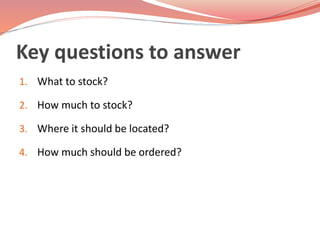
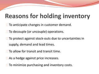
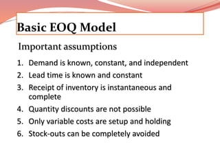
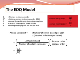
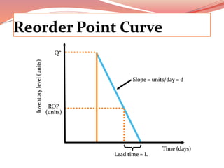
“Inventory Management” 
To hold or not to hold?
Objectives 
Appreciate the importance of effective inventory 
management. 
Understand the different reasons for holding inventory 
and the different types of inventory 
Describe the different costs of inventory. 
Realize the significance of independent and dependent 
demand in inventory control systems.
Objectives 
Be aware of the concept of Economic Order Quantity 
and its limitations. 
Describe the different inventory systems based on 
independent demand. 
Explain technologies as used for classifying and 
controlling inventory.
Introduction 
Inventory-A physical resource that a firm holds in stock 
with the intent of selling it or transforming it into a more 
valuable state. 
Inventory System- A set of policies and controls that 
monitors levels of inventory and determines what levels 
should be maintained, when stock should be replenished, 
and how large orders should be placed.
Inventory 
One of the most expensive assets of many companies, 
representing as much as 30-40% of total invested capital 
Operations managers must balance inventory 
investment and customer service
Inventory Management 
It is the planning and control of inventories (or stock) in 
the transformation system of an organization in order to 
meet customer demand while also being effective.
Key questions to answer 
1. What to stock? 
2. How much to stock? 
3. Where it should be located? 
4. How much should be ordered?
Reasons for holding inventory 
To anticipate changes in customer demand. 
To decouple (or uncouple) operations. 
To protect against stock-outs due to uncertainties in 
supply, demand and lead times. 
To allow for transit and transit time. 
As a hedge against price increases. 
To minimize purchasing and inventory costs.
Types of inventory 
Raw materials- all commodities, parts and 
components. 
MRO: Maintenance, Repairs and Operating Supplies 
Work-in-Process 
Finished Goods
The Costs of Inventory 
Ordering Costs (Including set-up costs) 
Holding costs (Capital costs, Storage costs, Insurance 
costs and obsolescence costs) 
Stock-out costs (costs involved in dealing with stock-outs)
Inventory systems based on Independent 
Demand 
Fixed-Order Quantity System (sometimes referred to as 
EOQ or Q systems). 
Fixed-time Period Systems(or Period Review system or 
Fixed order interval or P systems).
The Economic Order Quantity (EOQ) Model 
The EOQ is the order quantity that minimizes the 
ordering cost and the holding cost of an item i.e. 
minimizing the total costs in acquiring and holding 
assets
Basic EOQ Model 
Important assumptions 
1. Demand is known, constant, and independent 
2. Lead time is known and constant 
3. Receipt of inventory is instantaneous and 
complete 
4. Quantity discounts are not possible 
5. Only variable costs are setup and holding 
6. Stock-outs can be completely avoided
Inventory Usage Over Time 
Order quantity 
= Q (maximum 
inventory level) 
Inventory level 
Usage rate Average 
Time 
inventory on 
hand 
Q 
2 
Minimum 
inventory
Minimizing Costs 
Objective is to minimize total costs 
Annual cost 
Order quantity 
Curve for total 
cost of holding 
and setup 
Holding cost 
curve 
Setup (or order) 
cost curve 
Minimum 
total cost 
Optimal 
order 
quantity
The EOQ Model 
Q = Number of pieces per order 
Q* = Optimal number of pieces per order (EOQ) 
D = Annual demand in units for the Inventory item 
S = Setup or ordering cost for each order 
H = Holding or carrying cost per unit per year 
Annual setup cost = 
DS 
Q 
Annual holding cost = QH 
2 
Annual setup cost = (Number of orders placed per year) 
x (Setup or order cost per order) 
Annual demand 
Number of units in each order 
Setup or order 
cost per order 
= 
= D (S) 
Q
The EOQ Model 
Q = Number of pieces per order 
Q* = Optimal number of pieces per order (EOQ) 
D = Annual demand in units for the Inventory item 
S = Setup or ordering cost for each order 
H = Holding or carrying cost per unit per year 
Annual holding cost = (Average inventory level) 
x (Holding cost per unit per year) 
Order quantity 
= (Holding cost per unit per year) 
2 
= Q (H) 
2 
Annual setup cost = 
DS 
Q 
Annual holding cost = QH 
2
The EOQ Model 
Q = Number of pieces per order 
Q* = Optimal number of pieces per order (EOQ) 
D = Annual demand in units for the Inventory item 
S = Setup or ordering cost for each order 
H = Holding or carrying cost per unit per year 
Annual setup cost = 
DS 
Q 
Annual holding cost = QH 
2 
Optimal order quantity is found when annual setup cost equals 
annual holding cost 
D 
Q 
Q 
2 
S = H 
Solving for Q* 
2DS = Q2H 
Q2 = 2DS/H 
Q* = 2DS/H
An EOQ Example 
Determine optimal number of needles to order 
D = 1,000 units 
S = $10 per order 
H = $.50 per unit per year 
Q* = 
2DS 
H 
Q* = 
2(1,000)(10) 
0.50 
= 40,000 = 200 units
An EOQ Example 
Determine optimal number of needles to order 
D = 1,000 units Q* = 200 units 
S = $10 per order 
H = $.50 per unit per year 
= N = = 
Expected number 
of orders 
Demand 
Order quantity 
D 
Q* 
1,000 
200 
N = = 5 orders per year
An EOQ Example 
Determine optimal number of needles to order 
D = 1,000 units Q* = 200 units 
S = $10 per order N = 5 orders per year 
H = $.50 per unit per year 
= T = 
Expected time 
between orders 
Number of working 
days per year 
N 
T = 2 5 0 = 50 days between orders 
5
An EOQ Example 
Determine optimal number of needles to order 
D = 1,000 units Q* = 200 units 
S = $10 per order N = 5 orders per year 
H = $.50 per unit per year T = 50 days 
Total annual cost = Setup cost + Holding cost 
TC = D S + H 
Q 
Q 
2 
1,000 
200 
TC = ($10) + ($.50) 
200 
2 
TC = (5)($10) + (100)($.50) = $50 + $50 = $100
Robust Model 
 The EOQ model is robust 
 It works even if all parameters and 
assumptions are not met 
 The total cost curve is relatively flat in 
the area of the EOQ
Reorder Points 
 EOQ answers the “how much” question 
 The reorder point (ROP) tells when to order 
ROP = 
Lead time for a new 
order in days 
Demand 
per day 
= d x L 
d = D 
Number of working days in a year
Reorder Point Curve 
Q* 
ROP 
(units) 
Inventory level (units) 
Slope = units/day = d 
Time (days) 
Lead time = L
Reorder Point Example 
Demand = 8,000 DVDs per year 
250 working day year 
Lead time for orders is 3 working days 
d = 
ROP = d x L 
D 
Number of working days in a year 
= 8,000/250 = 32 units 
= 32 units per day x 3 days = 96 units
Fixed-time Period (P) Systems 
Here the inventory levels are reviewed at fixed intervals.
Four of the original EOQ assumptions maintained 
No constraints are placed on lot size 
Holding and ordering costs 
Independent demand 
Lead times are certain 
Order is placed to bring the inventory position up to the target 
inventory level, T, when the predetermined time, P, has elapsed
Fixed-time Period System(P) 
P P 
T 
L L L 
Protection interval 
Time 
On-hand inventory 
IP1 
IP3 
IP2 
Order 
placed 
Order 
placed 
Order 
received 
Order 
received 
Order 
received 
IP IP IP 
OH OH 
Q1 
Q2 
Q3 
P System When Demand Is Uncertain
Pareto Principle 
80/20 rule 
Based on the work of an economist & avid horticulturalist, 
V. Pareto in late 19th century Italy. 
80% of the land was owned by 20% of the people. 
80% of the peas were produced by 20% of the pods 
Applied to business by quality guru Dr. Juran
Pareto principle applied: 
Applied to Meetings: 80% of decisions come from 20% of 
meeting time. 
Applied to product defects: 20% of the quality problems cause 
80% of the defects. 
Applied to Salespeople: Roughly 20% of a sales force will 
develop 80% of the annual results 
Applied to Business Units: Roughly 20% of a company's business 
units will produce 80% of the annual revenue. 
Applied to time-management…
Moral of the Pareto principle 
Find the significant 20% 
Manage that 20%
Pareto principal + Inventory = ABC Analysis 
“critical few and the trivial many” 
Create a Pareto chart for the inventory dollars per year of 
each item – dollar-volume 
Generally the top 80% of dollars are from approximately 
20% of the items. 
Categorize all items into 
Class A items – top ~20% items by dollar-volume 
Class B items 
Class C items
10 20 30 40 50 60 70 80 90 100 
Percentage of items 
Percentage of dollar value 
100 — 
90 — 
80 — 
70 — 
60 — 
50 — 
40 — 
30 — 
20 — 
10 — 
0 —
10 20 30 40 50 60 70 80 90 100 
Percentage of items 
Percentage of dollar value 
100 — 
90 — 
80 — 
70 — 
60 — 
50 — 
40 — 
30 — 
20 — 
10 — 
0 —
10 20 30 40 50 60 70 80 90 100 
Percentage of items 
Percentage of dollar value 
100 — 
90 — 
80 — 
70 — 
60 — 
50 — 
40 — 
30 — 
20 — 
10 — 
0 —
10 20 30 40 50 60 70 80 90 100 
Percentage of items 
Percentage of dollar value 
100 — 
90 — 
80 — 
70 — 
60 — 
50 — 
40 — 
30 — 
20 — 
10 — 
0 —
10 20 30 40 50 60 70 80 90 100 
Percentage of items 
Percentage of dollar value 
100 — 
90 — 
80 — 
70 — 
60 — 
50 — 
40 — 
30 — 
20 — 
10 — 
0 — 
Class C 
Class A 
Class B
ABC Analysis 
Policies based on ABC analysis 
Develop Class A suppliers more 
Implement tighter physical control of Class 
A items 
Forecast Class A items more carefully 
Model inventory for Class A items
Cycle counting 
Physically counting a sample of total inventory on 
a regular basis 
Used often with ABC classification 
Class A items counted most often (e.g., daily) 
Class B items counted less frequently (e.g. weekly) 
Class C items counted least often (e.g. monthly)
Advantages of Cycle Counting 
Eliminates shutdown and interruption of production 
necessary for annual physical inventories 
Eliminates annual inventory adjustments 
Provides trained personnel to audit the accuracy of 
inventory 
Allows the cause of errors to be identified and 
remedial action to be taken 
Maintains accurate inventory records
Thank you

Inventory management

  • 1.
    “Inventory Management” Tohold or not to hold?
  • 2.
    Objectives Appreciate theimportance of effective inventory management. Understand the different reasons for holding inventory and the different types of inventory Describe the different costs of inventory. Realize the significance of independent and dependent demand in inventory control systems.
  • 3.
    Objectives Be awareof the concept of Economic Order Quantity and its limitations. Describe the different inventory systems based on independent demand. Explain technologies as used for classifying and controlling inventory.
  • 4.
    Introduction Inventory-A physicalresource that a firm holds in stock with the intent of selling it or transforming it into a more valuable state. Inventory System- A set of policies and controls that monitors levels of inventory and determines what levels should be maintained, when stock should be replenished, and how large orders should be placed.
  • 5.
    Inventory One ofthe most expensive assets of many companies, representing as much as 30-40% of total invested capital Operations managers must balance inventory investment and customer service
  • 6.
    Inventory Management Itis the planning and control of inventories (or stock) in the transformation system of an organization in order to meet customer demand while also being effective.
  • 7.
    Key questions toanswer 1. What to stock? 2. How much to stock? 3. Where it should be located? 4. How much should be ordered?
  • 8.
    Reasons for holdinginventory To anticipate changes in customer demand. To decouple (or uncouple) operations. To protect against stock-outs due to uncertainties in supply, demand and lead times. To allow for transit and transit time. As a hedge against price increases. To minimize purchasing and inventory costs.
  • 9.
    Types of inventory Raw materials- all commodities, parts and components. MRO: Maintenance, Repairs and Operating Supplies Work-in-Process Finished Goods
  • 10.
    The Costs ofInventory Ordering Costs (Including set-up costs) Holding costs (Capital costs, Storage costs, Insurance costs and obsolescence costs) Stock-out costs (costs involved in dealing with stock-outs)
  • 12.
    Inventory systems basedon Independent Demand Fixed-Order Quantity System (sometimes referred to as EOQ or Q systems). Fixed-time Period Systems(or Period Review system or Fixed order interval or P systems).
  • 13.
    The Economic OrderQuantity (EOQ) Model The EOQ is the order quantity that minimizes the ordering cost and the holding cost of an item i.e. minimizing the total costs in acquiring and holding assets
  • 14.
    Basic EOQ Model Important assumptions 1. Demand is known, constant, and independent 2. Lead time is known and constant 3. Receipt of inventory is instantaneous and complete 4. Quantity discounts are not possible 5. Only variable costs are setup and holding 6. Stock-outs can be completely avoided
  • 15.
    Inventory Usage OverTime Order quantity = Q (maximum inventory level) Inventory level Usage rate Average Time inventory on hand Q 2 Minimum inventory
  • 16.
    Minimizing Costs Objectiveis to minimize total costs Annual cost Order quantity Curve for total cost of holding and setup Holding cost curve Setup (or order) cost curve Minimum total cost Optimal order quantity
  • 17.
    The EOQ Model Q = Number of pieces per order Q* = Optimal number of pieces per order (EOQ) D = Annual demand in units for the Inventory item S = Setup or ordering cost for each order H = Holding or carrying cost per unit per year Annual setup cost = DS Q Annual holding cost = QH 2 Annual setup cost = (Number of orders placed per year) x (Setup or order cost per order) Annual demand Number of units in each order Setup or order cost per order = = D (S) Q
  • 18.
    The EOQ Model Q = Number of pieces per order Q* = Optimal number of pieces per order (EOQ) D = Annual demand in units for the Inventory item S = Setup or ordering cost for each order H = Holding or carrying cost per unit per year Annual holding cost = (Average inventory level) x (Holding cost per unit per year) Order quantity = (Holding cost per unit per year) 2 = Q (H) 2 Annual setup cost = DS Q Annual holding cost = QH 2
  • 19.
    The EOQ Model Q = Number of pieces per order Q* = Optimal number of pieces per order (EOQ) D = Annual demand in units for the Inventory item S = Setup or ordering cost for each order H = Holding or carrying cost per unit per year Annual setup cost = DS Q Annual holding cost = QH 2 Optimal order quantity is found when annual setup cost equals annual holding cost D Q Q 2 S = H Solving for Q* 2DS = Q2H Q2 = 2DS/H Q* = 2DS/H
  • 20.
    An EOQ Example Determine optimal number of needles to order D = 1,000 units S = $10 per order H = $.50 per unit per year Q* = 2DS H Q* = 2(1,000)(10) 0.50 = 40,000 = 200 units
  • 21.
    An EOQ Example Determine optimal number of needles to order D = 1,000 units Q* = 200 units S = $10 per order H = $.50 per unit per year = N = = Expected number of orders Demand Order quantity D Q* 1,000 200 N = = 5 orders per year
  • 22.
    An EOQ Example Determine optimal number of needles to order D = 1,000 units Q* = 200 units S = $10 per order N = 5 orders per year H = $.50 per unit per year = T = Expected time between orders Number of working days per year N T = 2 5 0 = 50 days between orders 5
  • 23.
    An EOQ Example Determine optimal number of needles to order D = 1,000 units Q* = 200 units S = $10 per order N = 5 orders per year H = $.50 per unit per year T = 50 days Total annual cost = Setup cost + Holding cost TC = D S + H Q Q 2 1,000 200 TC = ($10) + ($.50) 200 2 TC = (5)($10) + (100)($.50) = $50 + $50 = $100
  • 24.
    Robust Model The EOQ model is robust  It works even if all parameters and assumptions are not met  The total cost curve is relatively flat in the area of the EOQ
  • 25.
    Reorder Points EOQ answers the “how much” question  The reorder point (ROP) tells when to order ROP = Lead time for a new order in days Demand per day = d x L d = D Number of working days in a year
  • 26.
    Reorder Point Curve Q* ROP (units) Inventory level (units) Slope = units/day = d Time (days) Lead time = L
  • 27.
    Reorder Point Example Demand = 8,000 DVDs per year 250 working day year Lead time for orders is 3 working days d = ROP = d x L D Number of working days in a year = 8,000/250 = 32 units = 32 units per day x 3 days = 96 units
  • 28.
    Fixed-time Period (P)Systems Here the inventory levels are reviewed at fixed intervals.
  • 29.
    Four of theoriginal EOQ assumptions maintained No constraints are placed on lot size Holding and ordering costs Independent demand Lead times are certain Order is placed to bring the inventory position up to the target inventory level, T, when the predetermined time, P, has elapsed
  • 30.
    Fixed-time Period System(P) P P T L L L Protection interval Time On-hand inventory IP1 IP3 IP2 Order placed Order placed Order received Order received Order received IP IP IP OH OH Q1 Q2 Q3 P System When Demand Is Uncertain
  • 32.
    Pareto Principle 80/20rule Based on the work of an economist & avid horticulturalist, V. Pareto in late 19th century Italy. 80% of the land was owned by 20% of the people. 80% of the peas were produced by 20% of the pods Applied to business by quality guru Dr. Juran
  • 33.
    Pareto principle applied: Applied to Meetings: 80% of decisions come from 20% of meeting time. Applied to product defects: 20% of the quality problems cause 80% of the defects. Applied to Salespeople: Roughly 20% of a sales force will develop 80% of the annual results Applied to Business Units: Roughly 20% of a company's business units will produce 80% of the annual revenue. Applied to time-management…
  • 34.
    Moral of thePareto principle Find the significant 20% Manage that 20%
  • 35.
    Pareto principal +Inventory = ABC Analysis “critical few and the trivial many” Create a Pareto chart for the inventory dollars per year of each item – dollar-volume Generally the top 80% of dollars are from approximately 20% of the items. Categorize all items into Class A items – top ~20% items by dollar-volume Class B items Class C items
  • 36.
    10 20 3040 50 60 70 80 90 100 Percentage of items Percentage of dollar value 100 — 90 — 80 — 70 — 60 — 50 — 40 — 30 — 20 — 10 — 0 —
  • 37.
    10 20 3040 50 60 70 80 90 100 Percentage of items Percentage of dollar value 100 — 90 — 80 — 70 — 60 — 50 — 40 — 30 — 20 — 10 — 0 —
  • 38.
    10 20 3040 50 60 70 80 90 100 Percentage of items Percentage of dollar value 100 — 90 — 80 — 70 — 60 — 50 — 40 — 30 — 20 — 10 — 0 —
  • 39.
    10 20 3040 50 60 70 80 90 100 Percentage of items Percentage of dollar value 100 — 90 — 80 — 70 — 60 — 50 — 40 — 30 — 20 — 10 — 0 —
  • 40.
    10 20 3040 50 60 70 80 90 100 Percentage of items Percentage of dollar value 100 — 90 — 80 — 70 — 60 — 50 — 40 — 30 — 20 — 10 — 0 — Class C Class A Class B
  • 41.
    ABC Analysis Policiesbased on ABC analysis Develop Class A suppliers more Implement tighter physical control of Class A items Forecast Class A items more carefully Model inventory for Class A items
  • 42.
    Cycle counting Physicallycounting a sample of total inventory on a regular basis Used often with ABC classification Class A items counted most often (e.g., daily) Class B items counted less frequently (e.g. weekly) Class C items counted least often (e.g. monthly)
  • 43.
    Advantages of CycleCounting Eliminates shutdown and interruption of production necessary for annual physical inventories Eliminates annual inventory adjustments Provides trained personnel to audit the accuracy of inventory Allows the cause of errors to be identified and remedial action to be taken Maintains accurate inventory records
  • 44.