Chapter 5_OM

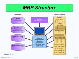
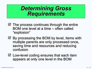
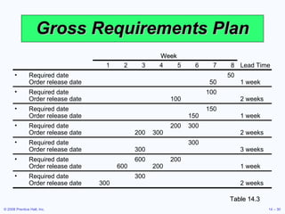
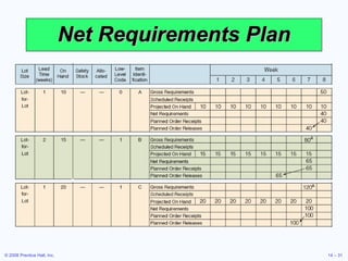
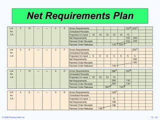
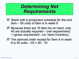
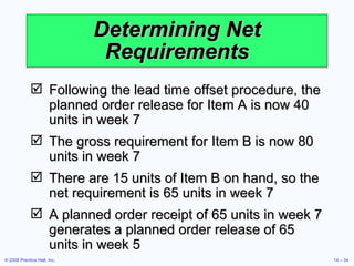
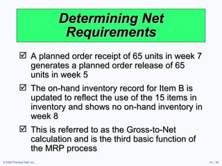
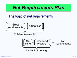
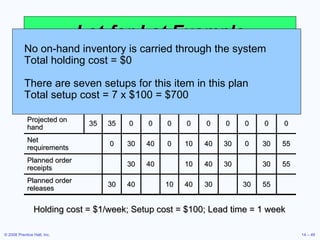
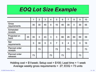
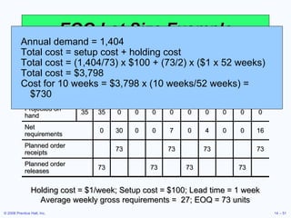
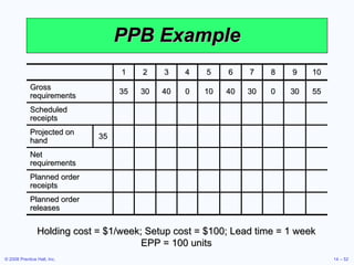
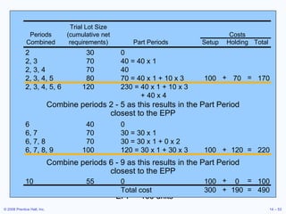
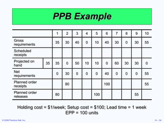
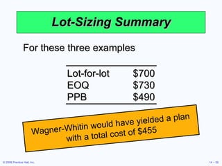
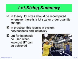
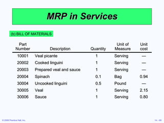
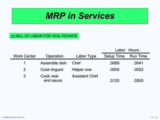
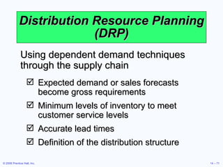
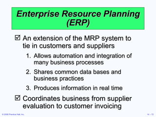
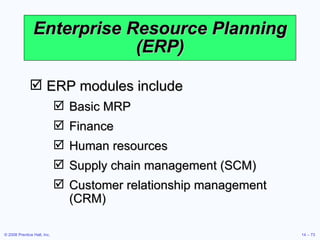
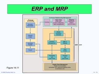
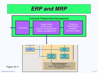
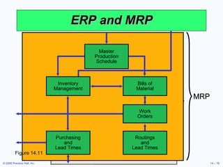
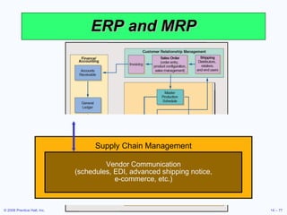
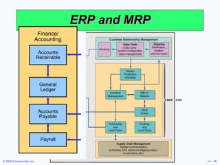
Operations Management Session 5 – Material Requirements Planning (MRP) and ERP

Learning Objectives When you complete this chapter you should be able to: Develop a product structure Build a gross requirements plan Build a net requirements plan Determine lot sizes for lot-for-lot, EOQ, and PPB

Learning Objectives When you complete this chapter you should be able to: Describe MRP II Describe closed-loop MRP Describe ERP

Wheeled Coach Largest manufacturer of ambulances in the world International competitor 12 major ambulance designs 18,000 different inventory items 6,000 manufactured parts 12,000 purchased parts

Wheeled Coach Four Key Tasks Material plan must meet both the requirements of the master schedule and the capabilities of the production facility Plan must be executed as designed Minimize inventory investment Maintain excellent record integrity

Benefits of MRP Better response to customer orders Faster response to market changes Improved utilization of facilities and labor Reduced inventory levels

Dependent Demand The demand for one item is related to the demand for another item Given a quantity for the end item, the demand for all parts and components can be calculated In general, used whenever a schedule can be established for an item MRP is the common technique

Dependent Demand Master production schedule Specifications or bill of material Inventory availability Purchase orders outstanding Lead times Effective use of dependent demand inventory models requires the following

Master Production Schedule (MPS) Specifies what is to be made and when Must be in accordance with the aggregate production plan Inputs from financial plans, customer demand, engineering, supplier performance As the process moves from planning to execution, each step must be tested for feasibility The MPS is the result of the production planning process

Master Production Schedule (MPS) MPS is established in terms of specific products Schedule must be followed for a reasonable length of time The MPS is quite often fixed or frozen in the near term part of the plan The MPS is a rolling schedule The MPS is a statement of what is to be produced, not a forecast of demand

The Planning Process Figure 14.1 Change production plan? Master production schedule Management Return on investment Capital Engineering Design completion Aggregate production plan Procurement Supplier performance Human resources Manpower planning Production Capacity Inventory Marketing Customer demand Finance Cash flow

The Planning Process Figure 14.1 Is capacity plan being met? Is execution meeting the plan? Change master production schedule? Change capacity? Change requirements? No Execute material plans Execute capacity plans Yes Realistic? Capacity requirements plan Material requirements plan Master production schedule

Aggregate Production Plan Figure 14.2 Months January February Aggregate Production Plan 1,500 1,200 (Shows the total quantity of amplifiers) Weeks 1 2 3 4 5 6 7 8 Master Production Schedule (Shows the specific type and quantity of amplifier to be produced 240-watt amplifier 100 100 100 100 150-watt amplifier 500 500 450 450 75-watt amplifier 300 100

Master Production Schedule (MPS) A customer order in a job shop (make-to-order) company Modules in a repetitive (assemble-to-order or forecast) company An end item in a continuous (stock-to-forecast) company Can be expressed in any of the following terms:

Focus for Different Process Strategies Figure 14.3 Stock to Forecast (Product Focus) Schedule finished product Assemble to Order or Forecast (Repetitive) Schedule modules Make to Order (Process Focus) Schedule orders Examples: Print shop Motorcycles Steel, Beer, Bread Machine shop Autos, TVs Lightbulbs Fine-dining restaurant Fast-food restaurant Paper Typical focus of the master production schedule Number of end items Number of inputs

MPS Examples Table 14.1 For Nancy’s Specialty Foods Gross Requirements for Crabmeat Quiche Gross Requirements for Spinach Quiche Day 6 7 8 9 10 11 12 13 14 and so on Amount 50 100 47 60 110 75 Day 7 8 9 10 11 12 13 14 15 16 and so on Amount 100 200 150 60 75 100

Bills of Material List of components, ingredients, and materials needed to make product Provides product structure Items above given level are called parents Items below given level are called children

BOM Example B (2) Std. 12” Speaker kit C (3) Std. 12” Speaker kit w/ amp-booster 1 E (2) E (2) F (2) Packing box and installation kit of wire, bolts, and screws Std. 12” Speaker booster assembly 2 D (2) 12” Speaker D (2) 12” Speaker G (1) Amp-booster 3 Product structure for “Awesome” (A) A Level 0

BOM Example Part B: 2 x number of As = (2)(50) = 100 Part C: 3 x number of As = (3)(50) = 150 Part D: 2 x number of Bs + 2 x number of Fs = (2)(100) + (2)(300) = 800 Part E: 2 x number of Bs + 2 x number of Cs = (2)(100) + (2)(150) = 500 Part F: 2 x number of Cs = (2)(150) = 300 Part G: 1 x number of Fs = (1)(300) = 300 B (2) Std. 12” Speaker kit C (3) Std. 12” Speaker kit w/ amp-booster 1 E (2) E (2) F (2) Packing box and installation kit of wire, bolts, and screws Std. 12” Speaker booster assembly 2 D (2) 12” Speaker D (2) 12” Speaker G (1) Amp-booster 3 Product structure for “Awesome” (A) A Level 0

Bills of Material Modular Bills Modules are not final products but components that can be assembled into multiple end items Can significantly simplify planning and scheduling

Bills of Material Planning Bills (Pseudo Bills) Created to assign an artificial parent to the BOM Used to group subassemblies to reduce the number of items planned and scheduled Used to create standard “kits” for production

Bills of Material Phantom Bills Describe subassemblies that exist only temporarily Are part of another assembly and never go into inventory Low-Level Coding Item is coded at the lowest level at which it occurs BOMs are processed one level at a time

Accurate Records Accurate inventory records are absolutely required for MRP (or any dependent demand system) to operate correctly Generally MRP systems require 99% accuracy Outstanding purchase orders must accurately reflect quantities and scheduled receipts

Lead Times The time required to purchase, produce, or assemble an item For production – the sum of the order, wait, move, setup, store, and run times For purchased items – the time between the recognition of a need and the availability of the item for production

Time-Phased Product Structure Figure 14.4 | | | | | | | | 1 2 3 4 5 6 7 8 Time in weeks F 2 weeks 3 weeks 1 week A 2 weeks 1 week D E 2 weeks D G 1 week 1 week 2 weeks to produce B C E Start production of D Must have D and E completed here so production can begin on B

MRP Structure Figure 14.5 Output Reports MRP by period report MRP by date report Planned order report Purchase advice Exception reports Order early or late or not needed Order quantity too small or too large Data Files Purchasing data BOM Lead times (Item master file) Inventory data Master production schedule Material requirement planning programs (computer and software)

Determining Gross Requirements Starts with a production schedule for the end item – 50 units of Item A in week 8 Using the lead time for the item, determine the week in which the order should be released – a 1 week lead time means the order for 50 units should be released in week 7 This step is often called “lead time offset” or “time phasing”

Determining Gross Requirements From the BOM, every Item A requires 2 Item Bs – 100 Item Bs are required in week 7 to satisfy the order release for Item A The lead time for the Item B is 2 weeks – release an order for 100 units of Item B in week 5 The timing and quantity for component requirements are determined by the order release of the parent(s)

Determining Gross Requirements The process continues through the entire BOM one level at a time – often called “explosion” By processing the BOM by level, items with multiple parents are only processed once, saving time and resources and reducing confusion Low-level coding ensures that each item appears at only one level in the BOM

Gross Requirements Plan Table 14.3 Week 1 2 3 4 5 6 7 8 Lead Time Required date 50 Order release date 50 1 week Required date 100 Order release date 100 2 weeks Required date 150 Order release date 150 1 week Required date 200 300 Order release date 200 300 2 weeks Required date 300 Order release date 300 3 weeks Required date 600 200 Order release date 600 200 1 week Required date 300 Order release date 300 2 weeks

Determining Net Requirements Starts with a production schedule for the end item – 50 units of Item A in week 8 Because there are 10 Item As on hand, only 40 are actually required – (net requirement) = (gross requirement - on- hand inventory) The planned order receipt for Item A in week 8 is 40 units – 40 = 50 - 10

Determining Net Requirements Following the lead time offset procedure, the planned order release for Item A is now 40 units in week 7 The gross requirement for Item B is now 80 units in week 7 There are 15 units of Item B on hand, so the net requirement is 65 units in week 7 A planned order receipt of 65 units in week 7 generates a planned order release of 65 units in week 5

Determining Net Requirements A planned order receipt of 65 units in week 7 generates a planned order release of 65 units in week 5 The on-hand inventory record for Item B is updated to reflect the use of the 15 items in inventory and shows no on-hand inventory in week 8 This is referred to as the Gross-to-Net calculation and is the third basic function of the MRP process

Net Requirements Plan The logic of net requirements Available inventory Net requirements On hand Scheduled receipts + – = Total requirements Gross requirements Allocations +

Gross Requirements Schedule Figure 14.6 A B C 5 6 7 8 9 10 11 40 50 15 Lead time = 4 for A Master schedule for A S B C 12 13 8 9 10 11 20 30 40 Lead time = 6 for S Master schedule for S 1 2 3 10 10 Master schedule for B sold directly Periods Therefore, these are the gross requirements for B Gross requirements: B 10 40 50 20 40+10 15+30 =50 =45 1 2 3 4 5 6 7 8 Periods

MRP Planning Sheet Figure 14.7

Safety Stock BOMs, inventory records, purchase and production quantities may not be perfect Consideration of safety stock may be prudent Should be minimized and ultimately eliminated Typically built into projected on-hand inventory

MRP Management MRP is a dynamic system Facilitates replanning when changes occur System nervousness can result from too many changes Time fences put limits on replanning Pegging links each item to its parent allowing effective analysis of changes

MRP and JIT MRP is a planning system that does not do detailed scheduling MRP requires fixed lead times which might actually vary with batch size JIT excels at rapidly moving small batches of material through the system

Finite Capacity Scheduling MRP systems do not consider capacity during normal planning cycles Finite capacity scheduling (FCS) recognizes actual capacity limits By merging MRP and FCS, a finite schedule is created with feasible capacities which facilitates rapid material movement

Small Bucket Approach MRP “buckets” are reduced to daily or hourly The most common planning period (time bucket) for MRP systems is weekly Planned receipts are used internally to sequence production Inventory is moved through the plant on a JIT basis Completed products are moved to finished goods inventory which reduces required quantities for subsequent planned orders Back flushing based on the BOM is used to deduct inventory that was used in production

Balanced Flow Used in repetitive operations MRP plans are executed using JIT techniques based on “pull” principles Flows are carefully balanced with small lot sizes

Supermarket Items used by many products are held in a common area often called a supermarket Items are withdrawn as needed Inventory is maintained using JIT systems and procedures Common items are not planned by the MRP system

Lot-Sizing Techniques Lot-for-lot techniques order just what is required for production based on net requirements May not always be feasible If setup costs are high, lot-for-lot can be expensive Economic order quantity (EOQ) EOQ expects a known constant demand and MRP systems often deal with unknown and variable demand

Lot-Sizing Techniques Part Period Balancing (PPB) looks at future orders to determine most economic lot size The Wagner-Whitin algorithm is a complex dynamic programming technique Assumes a finite time horizon Effective, but computationally burdensome

Lot-for-Lot Example Holding cost = $1/week; Setup cost = $100; Lead time = 1 week 1 2 3 4 5 6 7 8 9 10 Gross requirements 35 30 40 0 10 40 30 0 30 55 Scheduled receipts Projected on hand 35 35 0 0 0 0 0 0 0 0 0 Net requirements 0 30 40 0 10 40 30 0 30 55 Planned order receipts 30 40 10 40 30 30 55 Planned order releases 30 40 10 40 30 30 55

Lot-for-Lot Example Holding cost = $1/week; Setup cost = $100; Lead time = 1 week No on-hand inventory is carried through the system Total holding cost = $0 There are seven setups for this item in this plan Total setup cost = 7 x $100 = $700 1 2 3 4 5 6 7 8 9 10 Gross requirements 35 30 40 0 10 40 30 0 30 55 Scheduled receipts Projected on hand 35 35 0 0 0 0 0 0 0 0 0 Net requirements 0 30 40 0 10 40 30 0 30 55 Planned order receipts 30 40 10 40 30 30 55 Planned order releases 30 40 10 40 30 30 55

EOQ Lot Size Example Holding cost = $1/week; Setup cost = $100; Lead time = 1 week Average weekly gross requirements = 27; EOQ = 73 units 1 2 3 4 5 6 7 8 9 10 Gross requirements 35 30 40 0 10 40 30 0 30 55 Scheduled receipts Projected on hand 35 35 0 43 3 3 66 26 69 69 39 Net requirements 0 30 0 0 7 0 4 0 0 16 Planned order receipts 73 73 73 73 Planned order releases 73 73 73 73

EOQ Lot Size Example Holding cost = $1/week; Setup cost = $100; Lead time = 1 week Average weekly gross requirements = 27; EOQ = 73 units Annual demand = 1,404 Total cost = setup cost + holding cost Total cost = (1,404/73) x $100 + (73/2) x ($1 x 52 weeks) Total cost = $3,798 Cost for 10 weeks = $3,798 x (10 weeks/52 weeks) = $730 1 2 3 4 5 6 7 8 9 10 Gross requirements 35 30 40 0 10 40 30 0 30 55 Scheduled receipts Projected on hand 35 35 0 0 0 0 0 0 0 0 0 Net requirements 0 30 0 0 7 0 4 0 0 16 Planned order receipts 73 73 73 73 Planned order releases 73 73 73 73

PPB Example Holding cost = $1/week; Setup cost = $100; Lead time = 1 week EPP = 100 units 1 2 3 4 5 6 7 8 9 10 Gross requirements 35 30 40 0 10 40 30 0 30 55 Scheduled receipts Projected on hand 35 Net requirements Planned order receipts Planned order releases

PPB Example Holding cost = $1/week; Setup cost = $100; EPP = 100 units 1 2 3 4 5 6 7 8 9 10 Gross requirements 35 30 40 0 10 40 30 0 30 55 Scheduled receipts Projected on hand 35 Net requirements Planned order receipts Planned order releases 2 30 0 2, 3 70 40 = 40 x 1 2, 3, 4 70 40 2, 3, 4, 5 80 70 = 40 x 1 + 10 x 3 100 70 170 2, 3, 4, 5, 6 120 230 = 40 x 1 + 10 x 3 + 40 x 4 + = Combine periods 2 - 5 as this results in the Part Period closest to the EPP Combine periods 6 - 9 as this results in the Part Period closest to the EPP 6 40 0 6, 7 70 30 = 30 x 1 6, 7, 8 70 30 = 30 x 1 + 0 x 2 6, 7, 8, 9 100 120 = 30 x 1 + 30 x 3 100 120 220 + = 10 55 0 100 0 100 Total cost 300 190 490 + = + = Trial Lot Size Periods (cumulative net Costs Combined requirements) Part Periods Setup Holding Total

PPB Example Holding cost = $1/week; Setup cost = $100; Lead time = 1 week EPP = 100 units 1 2 3 4 5 6 7 8 9 10 Gross requirements 35 30 40 0 10 40 30 0 30 55 Scheduled receipts Projected on hand 35 35 0 50 10 10 0 60 30 30 0 Net requirements 0 30 0 0 0 40 0 0 0 55 Planned order receipts 80 100 55 Planned order releases 80 100 55

Lot-Sizing Summary For these three examples Wagner-Whitin would have yielded a plan with a total cost of $455 Lot-for-lot $700 EOQ $730 PPB $490

Lot-Sizing Summary In theory, lot sizes should be recomputed whenever there is a lot size or order quantity change In practice, this results in system nervousness and instability Lot-for-lot should be used when low-cost JIT can be achieved

Lot-Sizing Summary Lot sizes can be modified to allow for scrap, process constraints, and purchase lots Use lot-sizing with care as it can cause considerable distortion of requirements at lower levels of the BOM When setup costs are significant and demand is reasonably smooth, PPB, Wagner-Whitin, or EOQ should give reasonable results

Extensions of MRP Closed-Loop MRP MRP system provides input to the capacity plan, MPS, and production planning process Capacity Planning MRP system generates a load report which details capacity requirements This is used to drive the capacity planning process Changes pass back through the MRP system for rescheduling

Material Requirements Planning II Once an MRP system is in place, inventory data can be augmented by other useful information Labor hours Material costs Capital costs Virtually any resource System is generally called MRP II or Material Resource Planning

Material Resource Planning Table 14.4 Week 5 6 7 8 Units (lead time 1 week) 100 Labor: 10 hours each 1,000 Machine: 2 hours each 200 Payable: $0 each 0 Units (lead time 2 weeks, 2 each required) 200 Labor: 10 hours each 2,000 Machine: 2 hours each 400 Payable: Raw material at $5 each 1,000 Units (lead time 4 weeks, 3 each required) 300 Labor: 2 hours each 600 Machine: 1 hour each 300 Payable: Raw material at $10 each 3,000

Closed-Loop MRP System Figure 14.8

Closed-Loop MRP System Figure 14.8 Capacity Planning Resource planning First cut capacity No Capacity requirements (detailed) Yes Material requirements (detailed) Priority Planning Desired master production schedule Realistic? Production plan Planning

Closed-Loop MRP System Figure 14.8 Capacity Control (work center throughput) Priority Control (detailed scheduling) Execution Yes Execute the plan No No Input/output report Is average capacity adequate ? Dispatch list Is specific capacity adequate ?

Resource Requirements Profile Figure 14.9 Lot 1 Lot 2 Lot 4 Lot 7 Lot 8 Lot 3 Lot 5 Lot 10 Lot 13 Lot 9 Lot 12 Lot 14 Lot 16 Lot 6 Lot 15 Lot 11 Available capacity Capacity exceeded in periods 4 & 6 Lot 1 Lot 2 Lot 4 Lot 7 Lot 8 Lot 3 Lot 5 Lot 10 Lot 13 Lot 9 Lot 12 Lot 14 Lot 16 Lot 6 Lot 15 Lot 11 Available capacity Lot 6 “split” Lot 11 moved 200 – 150 – 100 – 50 – – 1 2 3 4 5 6 7 8 Period (a) Standard labor hours 200 – 150 – 100 – 50 – – 1 2 3 4 5 6 7 8 Period (b) Standard labor hours

Resource Requirements Profile It is also possible to split lots 6 and 11 and move them earlier in the schedule. This would avoid any potential problems with late orders but would increase inventory holding cost. Figure 14.9 Lot 1 Lot 2 Lot 4 Lot 7 Lot 8 Lot 3 Lot 5 Lot 10 Lot 13 Lot 9 Lot 12 Lot 14 Lot 16 Lot 6 Lot 15 Lot 11 Available capacity Capacity exceeded in periods 4 & 6 Lot 1 Lot 2 Lot 4 Lot 7 Lot 8 Lot 3 Lot 5 Lot 10 Lot 13 Lot 9 Lot 12 Lot 14 Lot 16 Lot 6 Lot 15 Lot 11 Available capacity Lot 6 “split” Lot 11 moved 200 – 150 – 100 – 50 – – 1 2 3 4 5 6 7 8 Period (a) Standard labor hours 200 – 150 – 100 – 50 – – 1 2 3 4 5 6 7 8 Period (b) Standard labor hours

Smoothing Tactics Overlapping Sends part of the work to following operations before the entire lot is complete Reduces lead time Operations splitting Sends the lot to two different machines for the same operation Shorter throughput time but increased setup costs Order or lot splitting Breaking up the order into smaller lots and running part ahead of schedule

MRP in Services Some services or service items are directly linked to demand for other services These can be treated as dependent demand services or items Restaurants Hospitals Hotels

MRP in Services (a) PRODUCT STRUCTURE TREE Figure 14.10 Uncooked linguini #30004 Sauce #30006 Veal #30005 Chef; Work Center #1 Helper one; Work Center #2 Asst. Chef; Work Center #3 Cooked linguini #20002 Spinach #20004 Prepared veal and sauce #20003 Veal picante #10001

MRP in Services (b) BILL OF MATERIALS Part Number Description Quantity Unit of Measure Unit cost 10001 Veal picante 1 Serving — 20002 Cooked linguini 1 Serving — 20003 Prepared veal and sauce 1 Serving — 20004 Spinach 0.1 Bag 0.94 30004 Uncooked linguini 0.5 Pound — 30005 Veal 1 Serving 2.15 30006 Sauce 1 Serving 0.80

MRP in Services (c) BILL OF LABOR FOR VEAL PICANTE Labor Hours Work Center Operation Labor Type Setup Time Run Time 1 Assemble dish Chef .0069 .0041 2 Cook linguini Helper one .0005 .0022 3 Cook veal and sauce Assistant Chef .0125 .0500

Distribution Resource Planning (DRP) Using dependent demand techniques through the supply chain Expected demand or sales forecasts become gross requirements Minimum levels of inventory to meet customer service levels Accurate lead times Definition of the distribution structure

Enterprise Resource Planning (ERP) An extension of the MRP system to tie in customers and suppliers Allows automation and integration of many business processes Shares common data bases and business practices Produces information in real time Coordinates business from supplier evaluation to customer invoicing

Enterprise Resource Planning (ERP) ERP modules include Basic MRP Finance Human resources Supply chain management (SCM) Customer relationship management (CRM)

ERP and MRP Figure 14.11 Customer Relationship Management Invoicing Shipping Distributors, retailers, and end users Sales Order (order entry, product configuration, sales management)

ERP and MRP Figure 14.11 Table 13.6 Bills of Material Work Orders Purchasing and Lead Times Routings and Lead Times Master Production Schedule Inventory Management MRP

ERP and MRP Figure 14.11 Supply Chain Management Vendor Communication (schedules, EDI, advanced shipping notice, e-commerce, etc.)

ERP and MRP Figure 14.11 Table 13.6 Finance/ Accounting General Ledger Accounts Receivable Payroll Accounts Payable

Enterprise Resource Planning (ERP) ERP can be highly customized to meet specific business requirements Enterprise application integration software (EAI) allows ERP systems to be integrated with Warehouse management Logistics Electronic catalogs Quality management

Enterprise Resource Planning (ERP) ERP systems have the potential to Reduce transaction costs Increase the speed and accuracy of information Facilitates a strategic emphasis on JIT systems and integration

Advantages of ERP Systems Provides integration of the supply chain, production, and administration Creates commonality of databases Can incorporate improved best processes Increases communication and collaboration between business units and sites Has an off-the-shelf software database May provide a strategic advantage

Disadvantages of ERP Systems Is very expensive to purchase and even more so to customize Implementation may require major changes in the company and its processes Is so complex that many companies cannot adjust to it Involves an ongoing, possibly never completed, process for implementation Expertise is limited with ongoing staffing problems

ERP in the Service Sector ERP systems have been developed for health care, government, retail stores, hotels, and financial services Also called efficient consumer response (ECR) systems Objective is to tie sales to buying, inventory, logistics, and production

Chapter 5_OM

More Related Content

What's hot

Viewers also liked

Similar to Chapter 5_OM

Recently uploaded

Chapter 5_OM