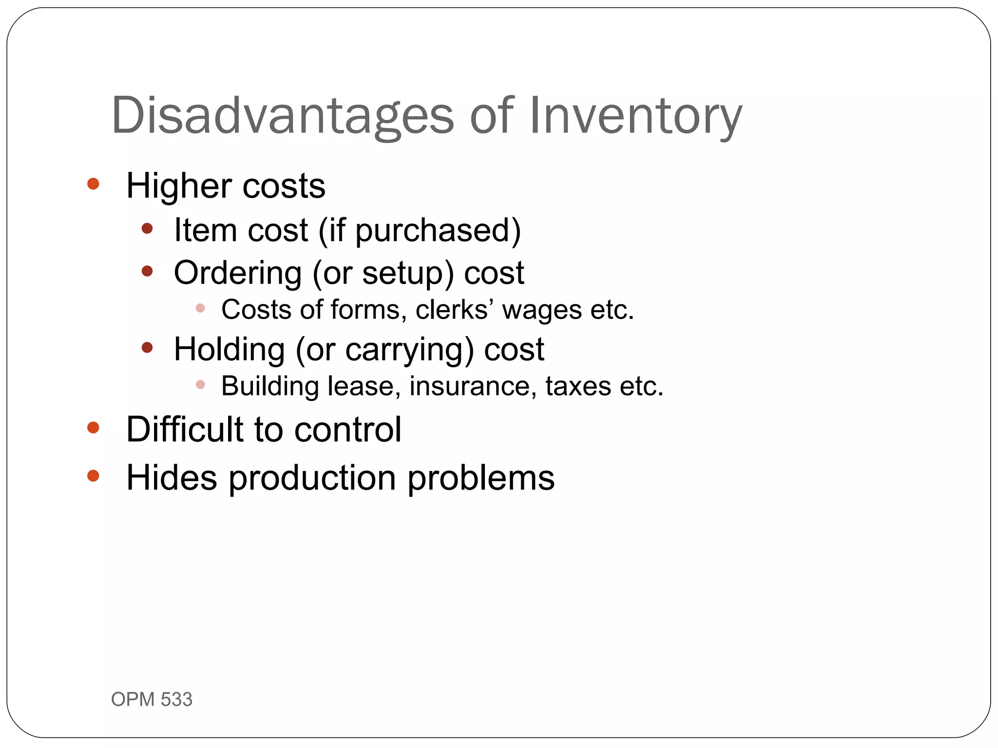
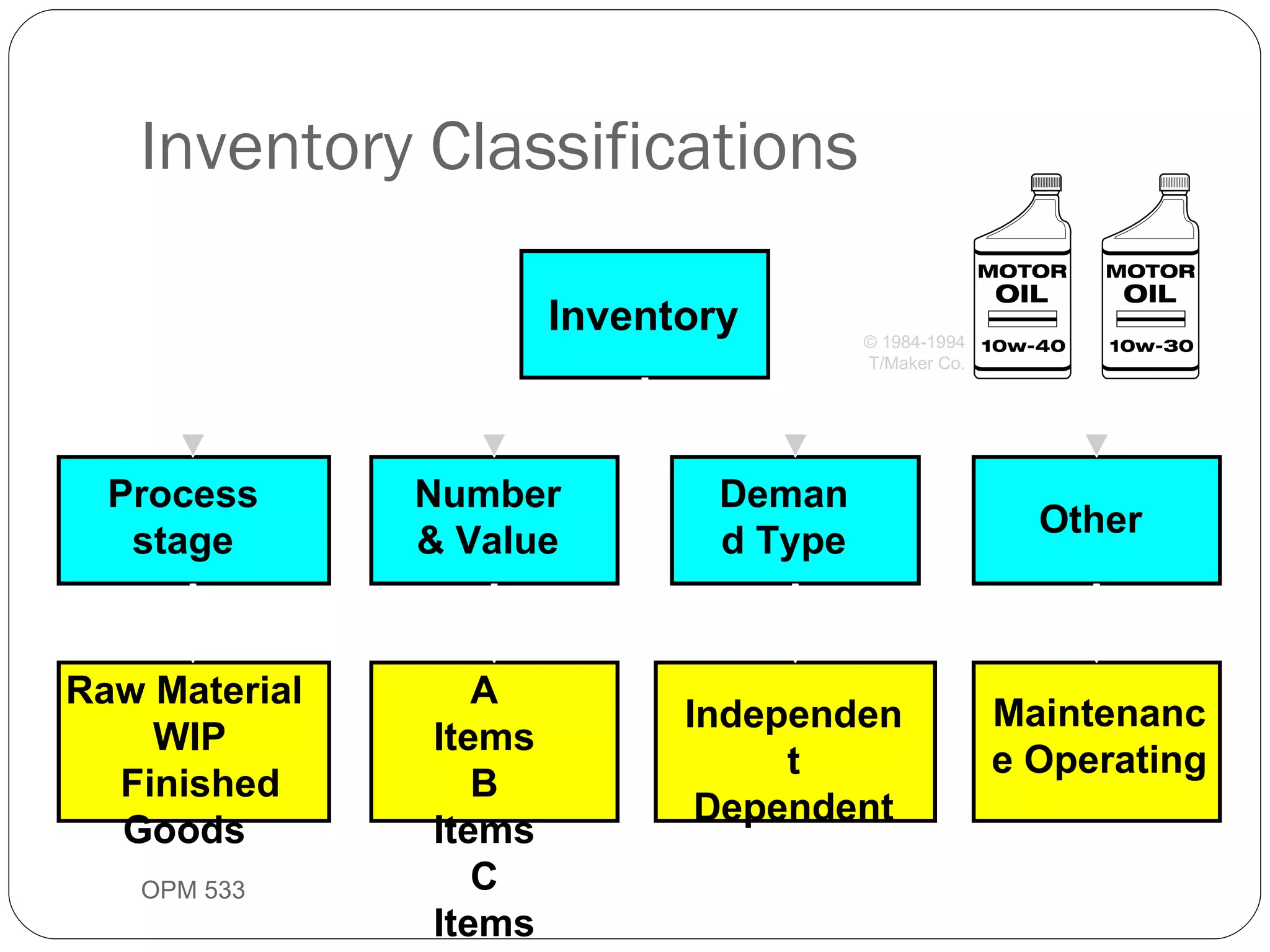
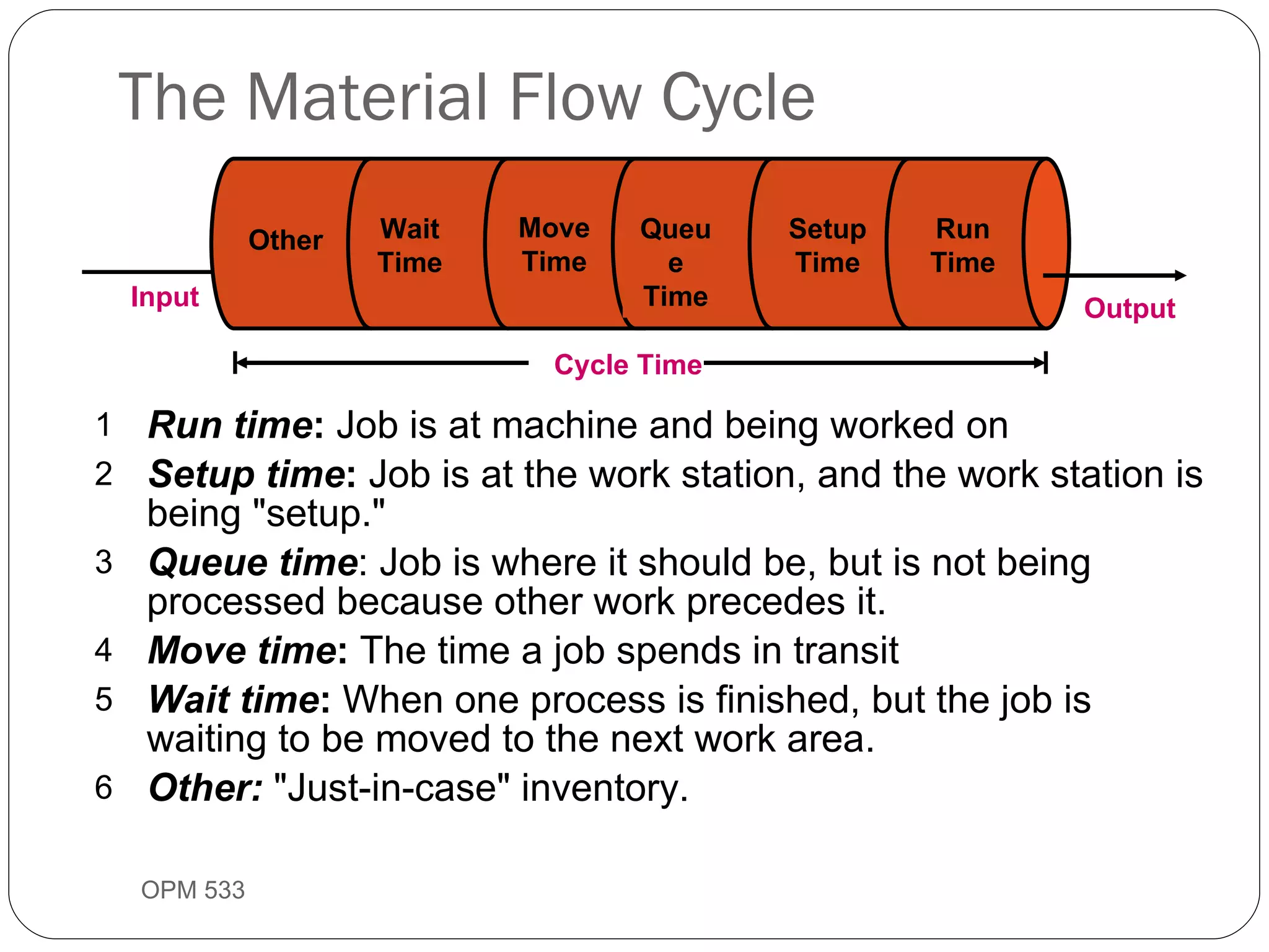
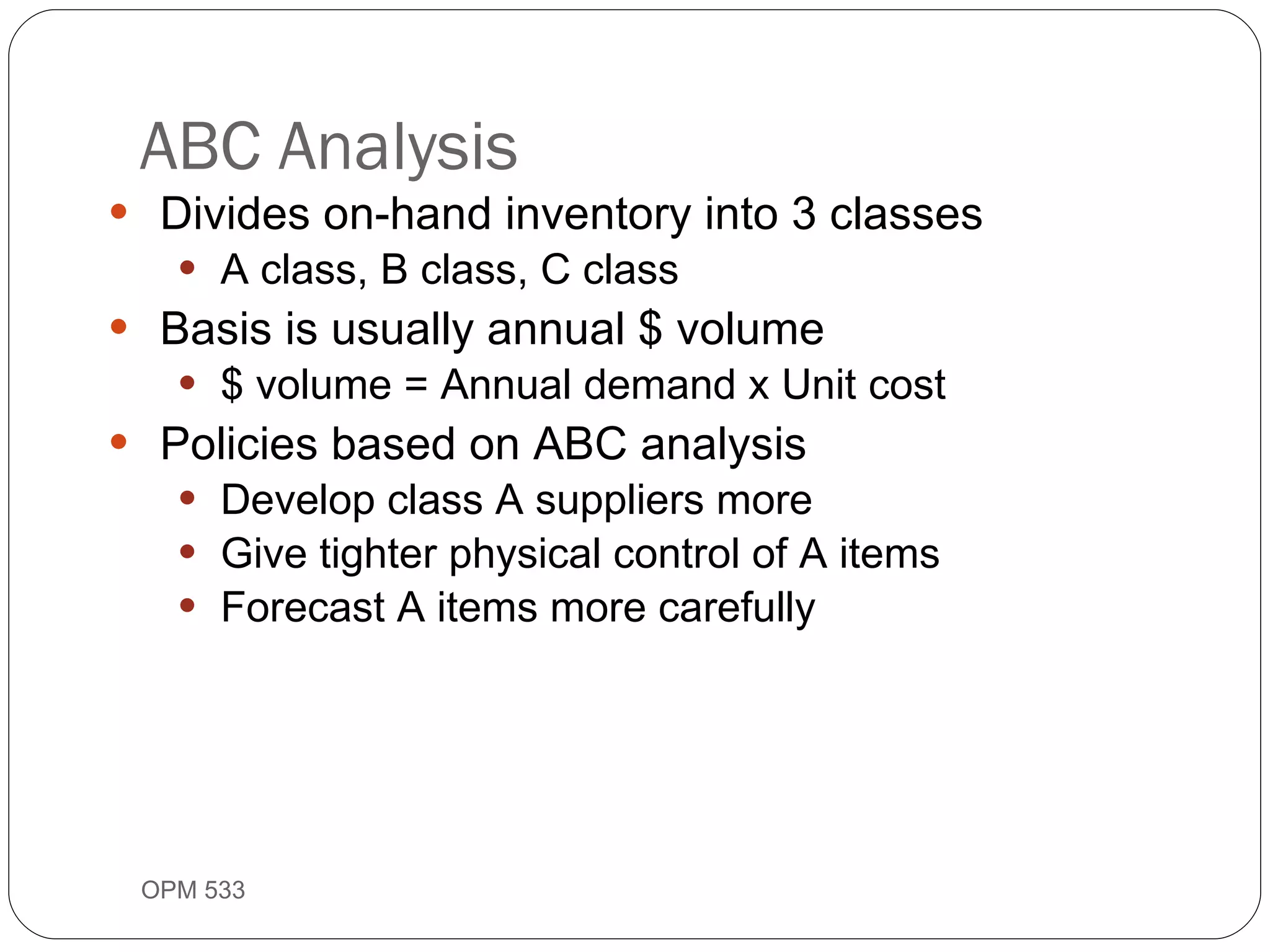
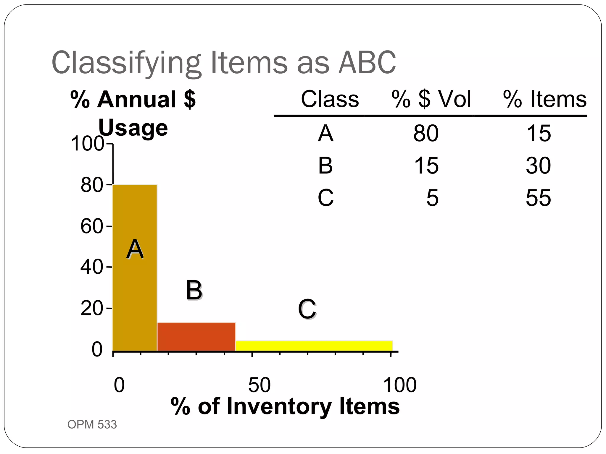
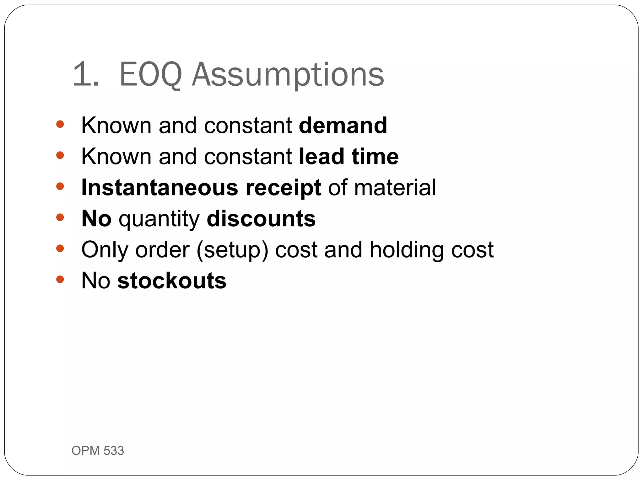
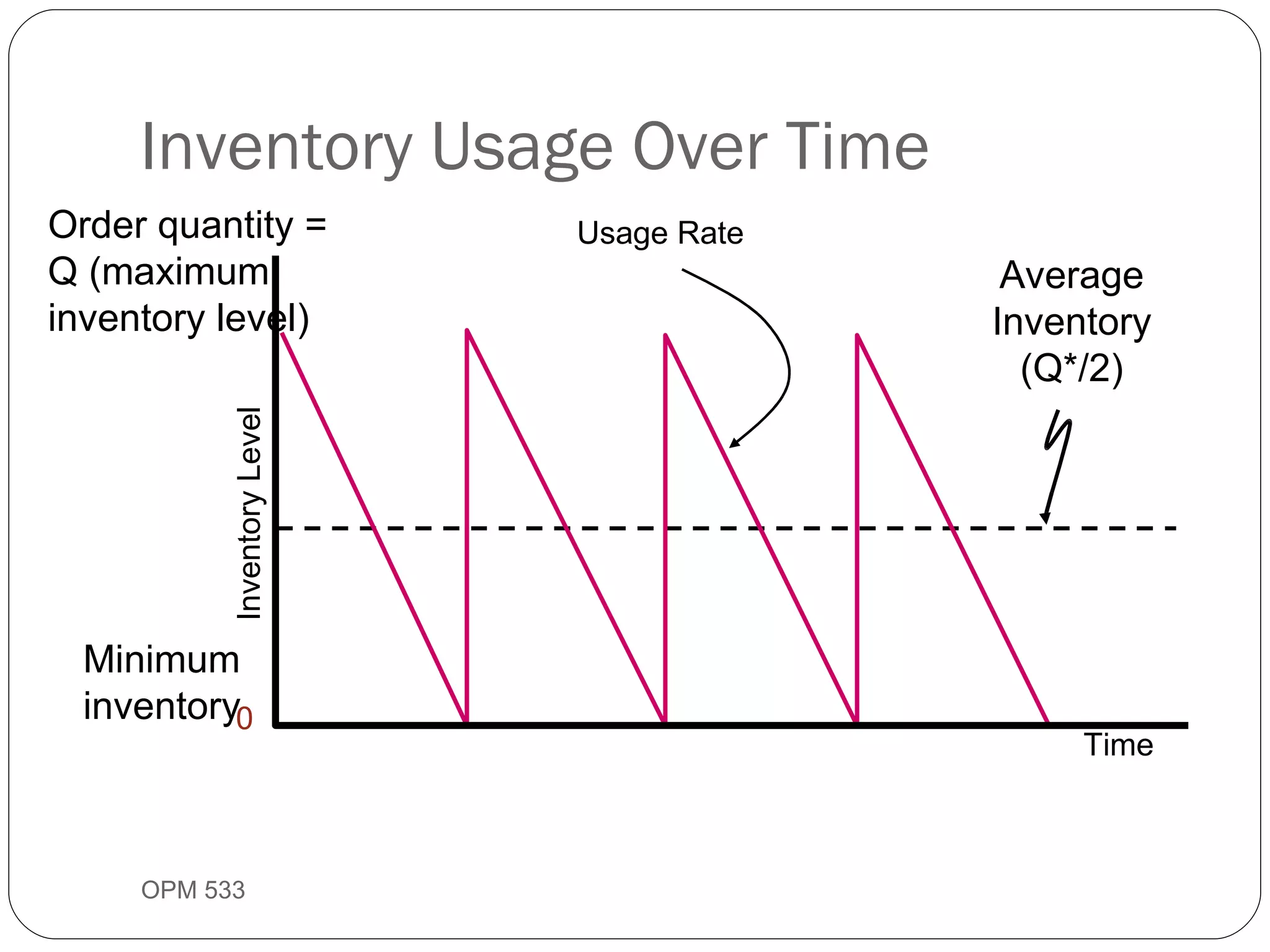
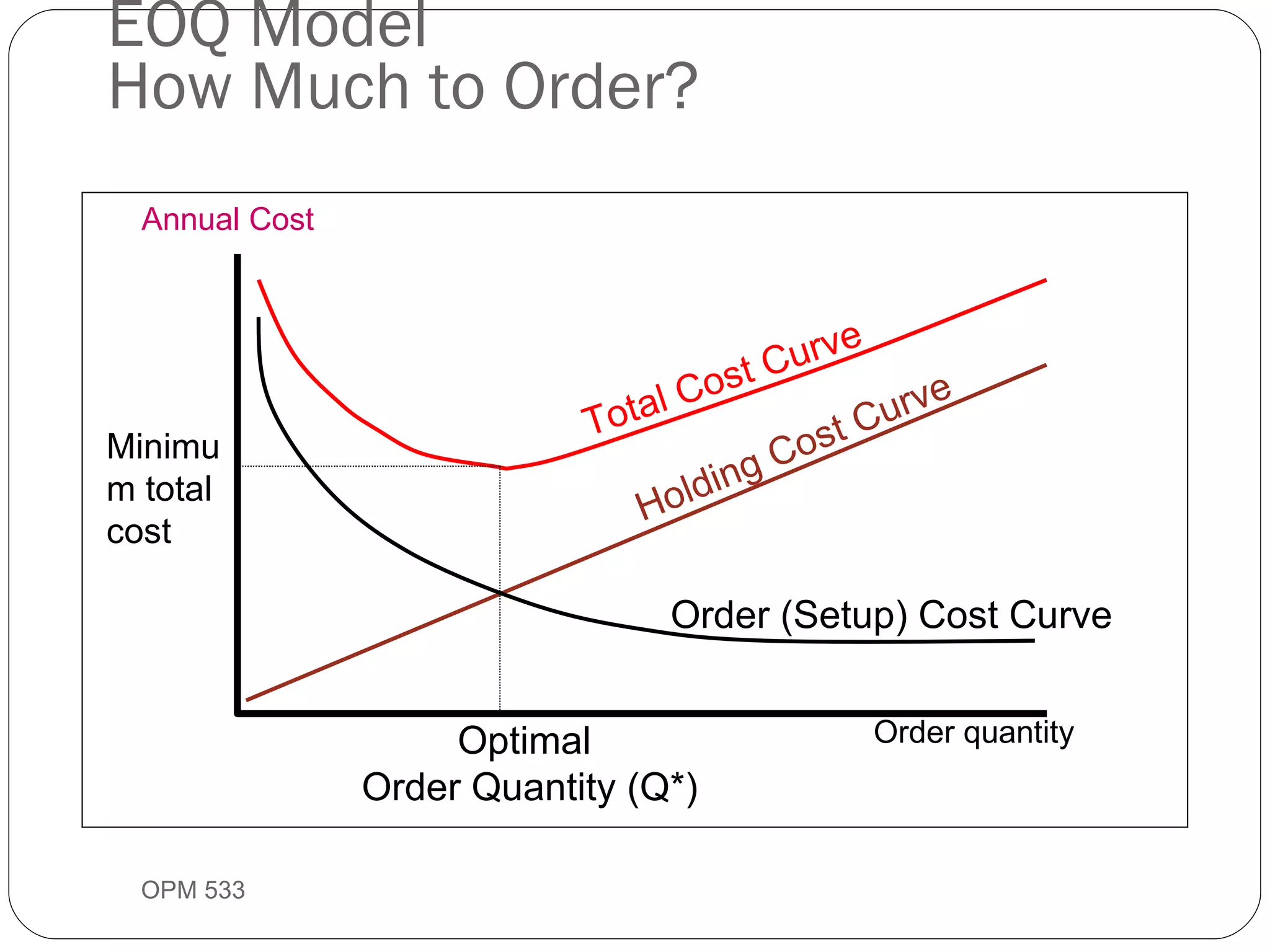
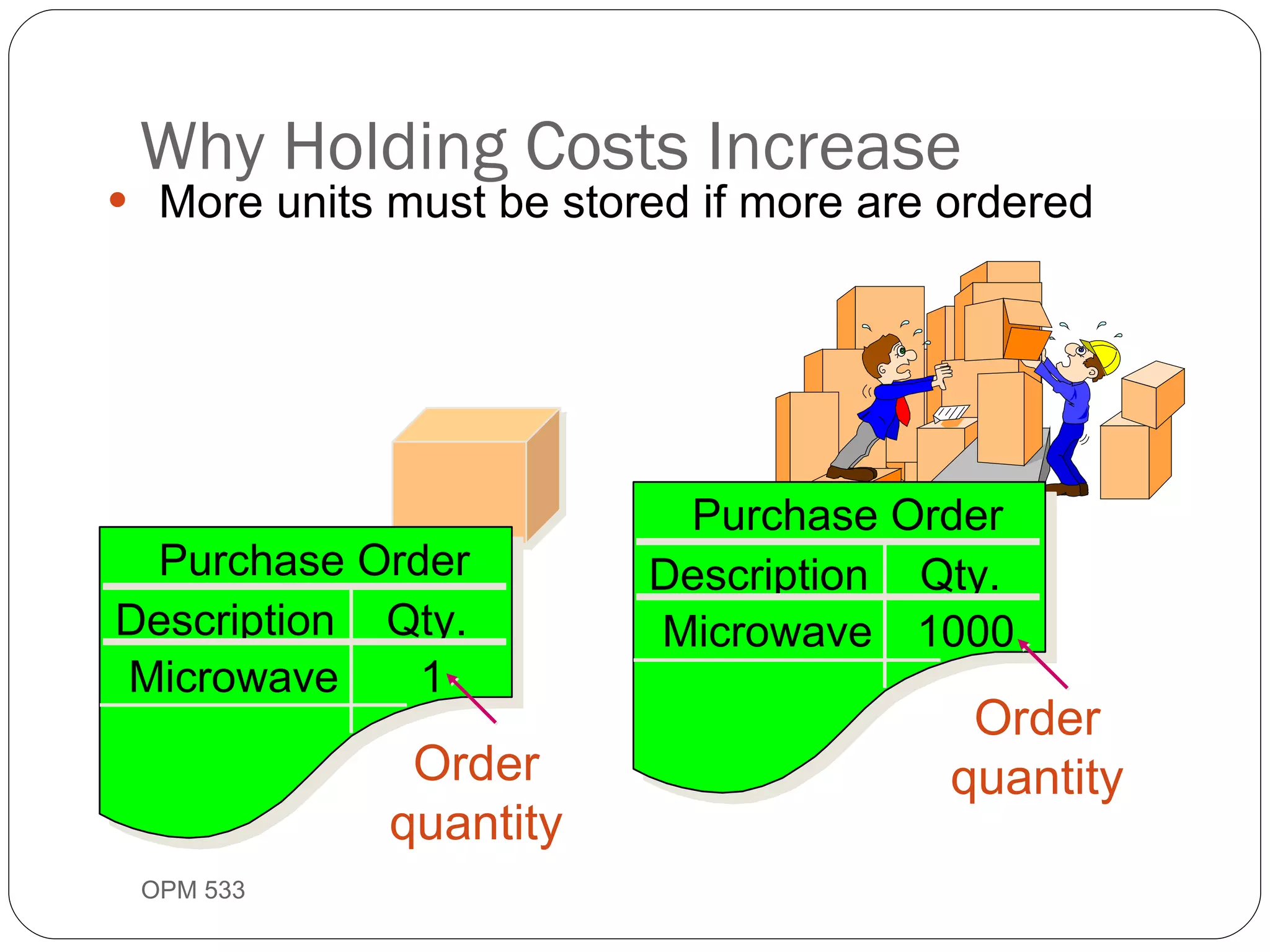
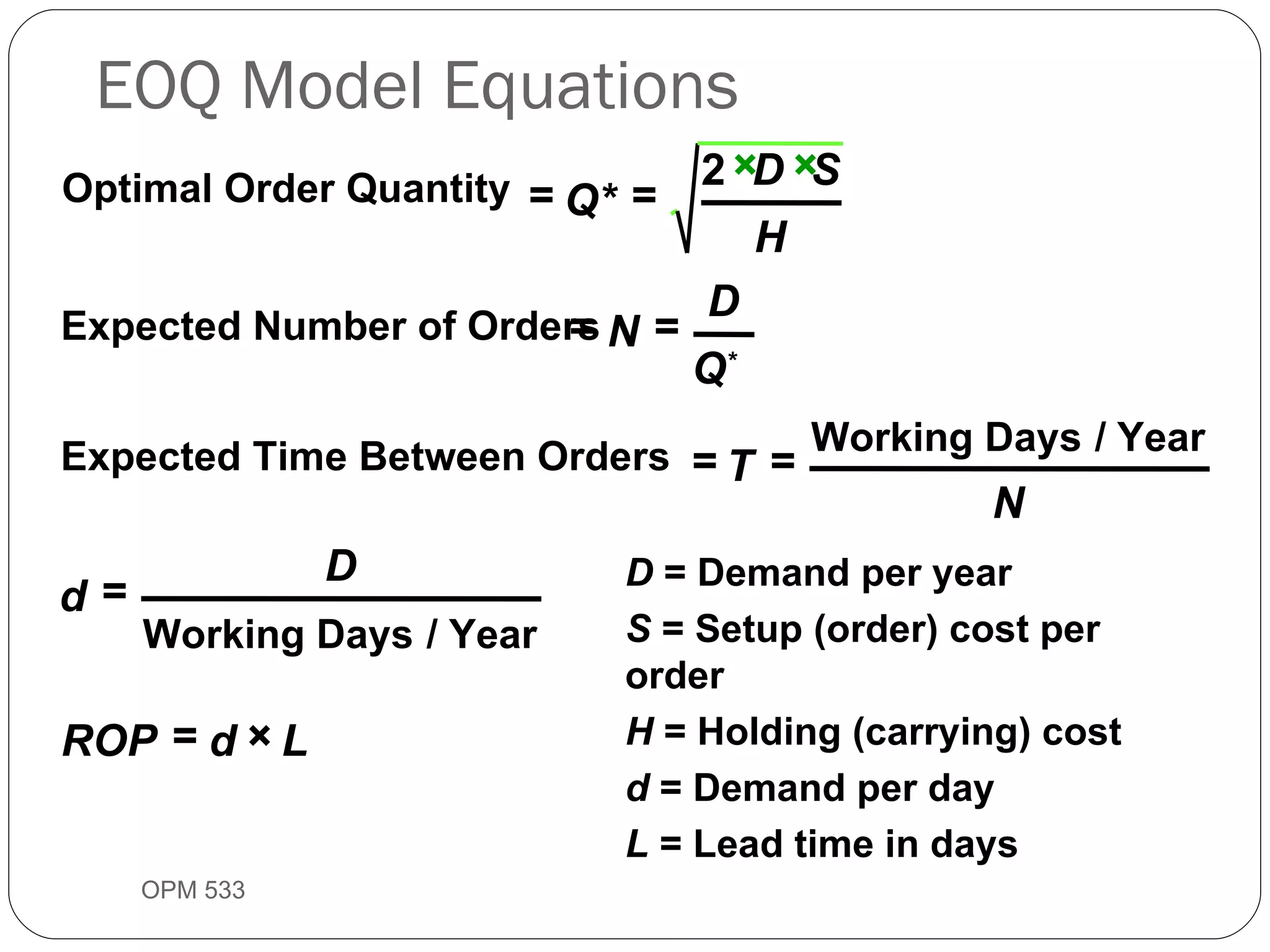
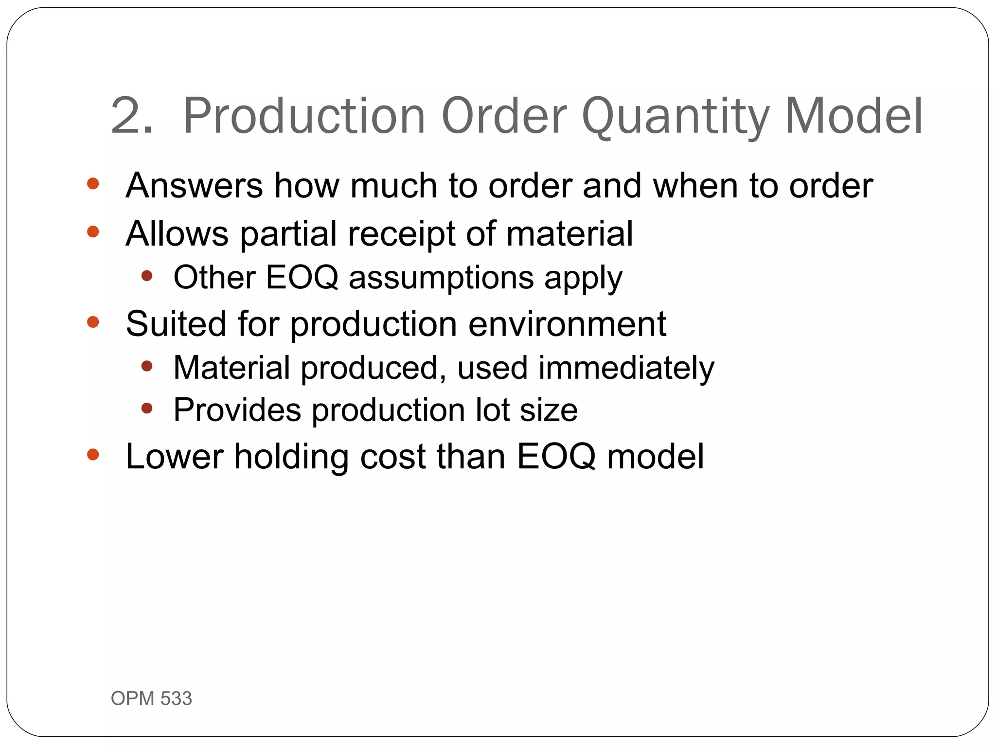
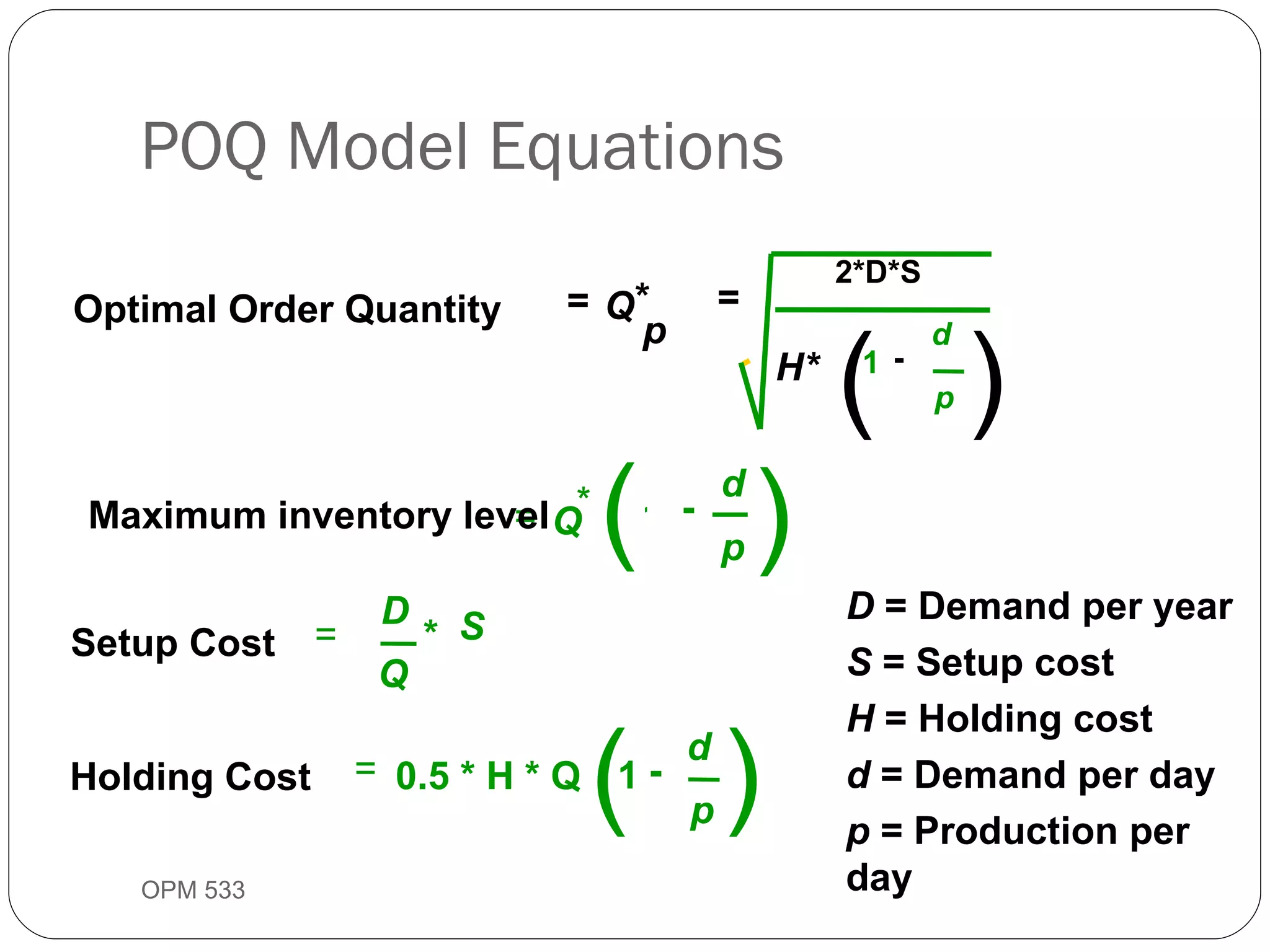
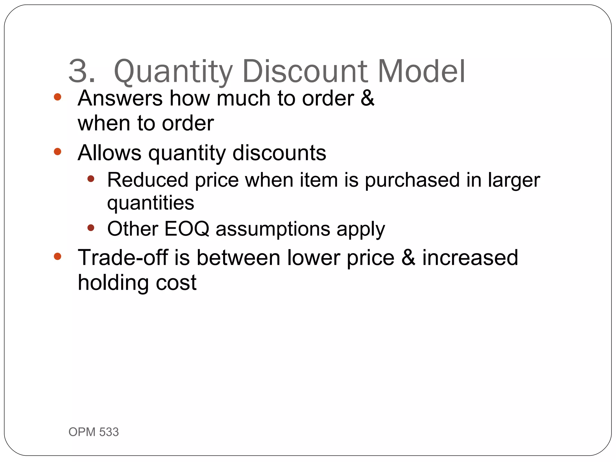
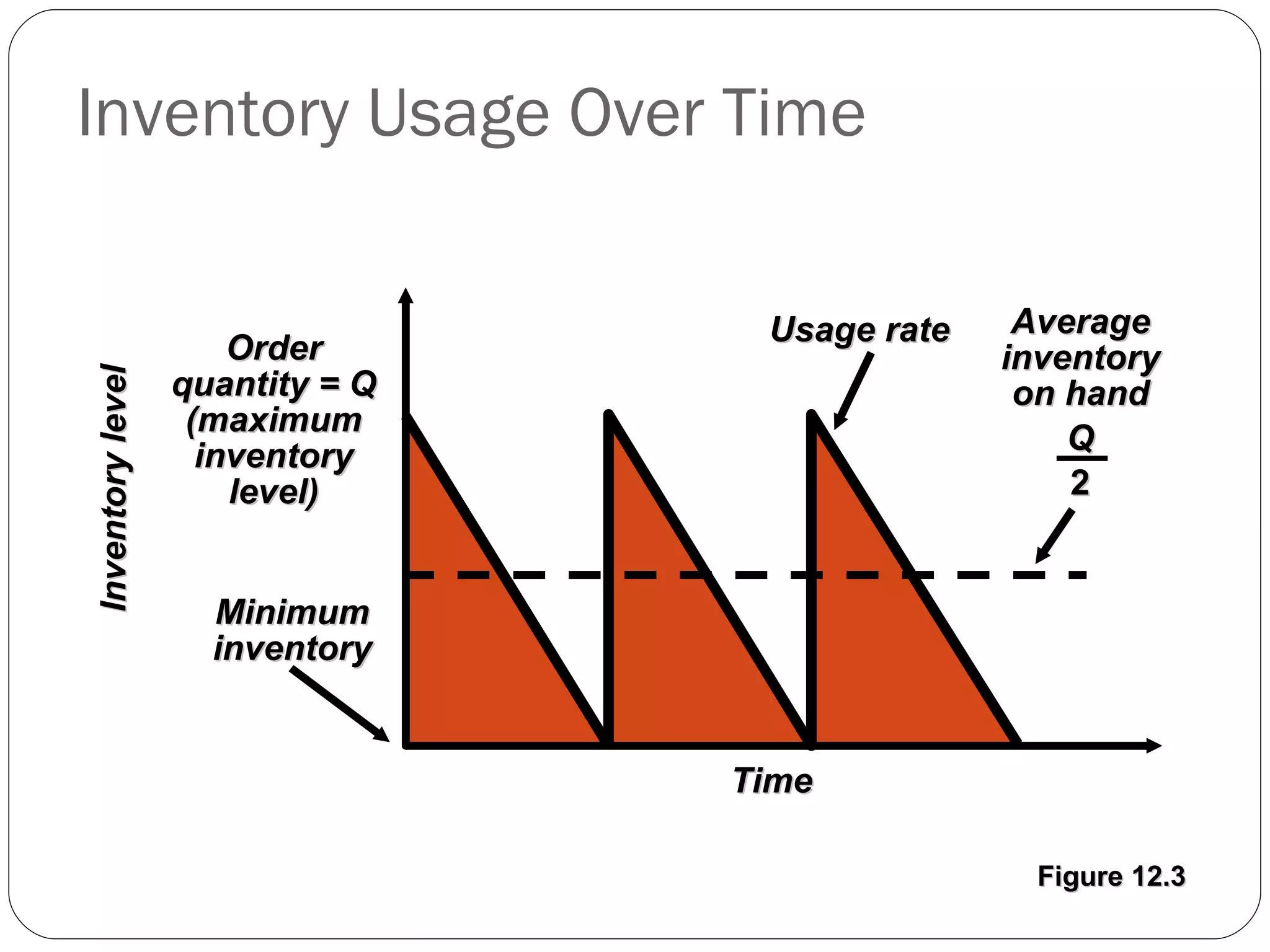
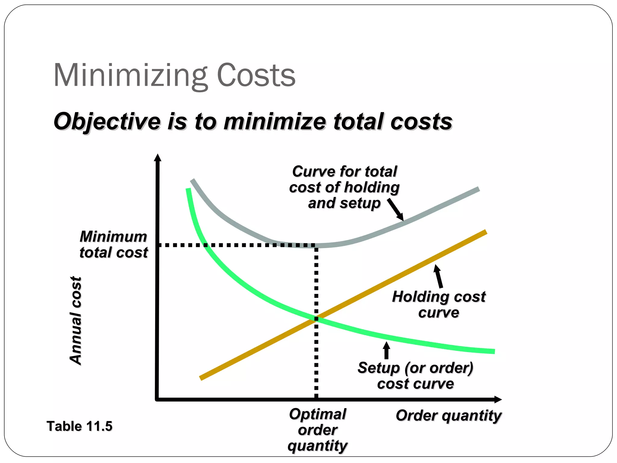
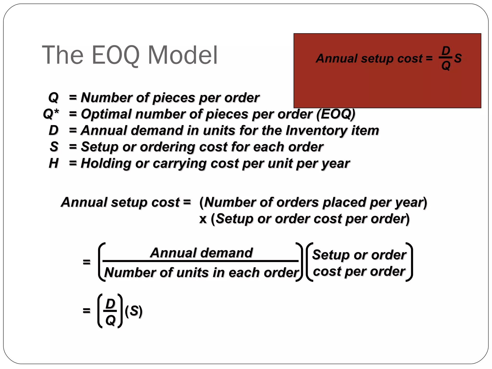
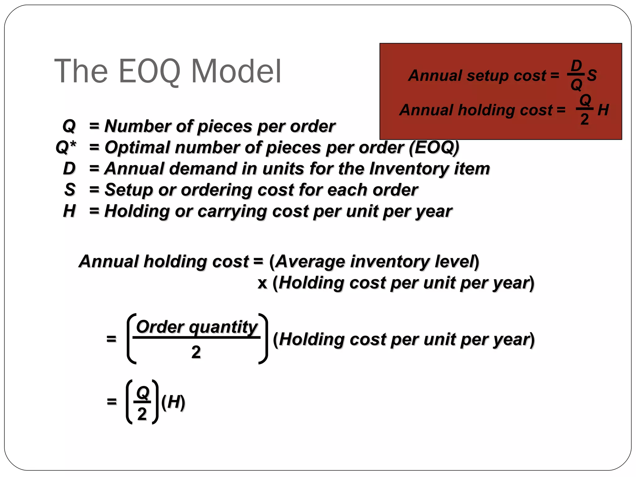
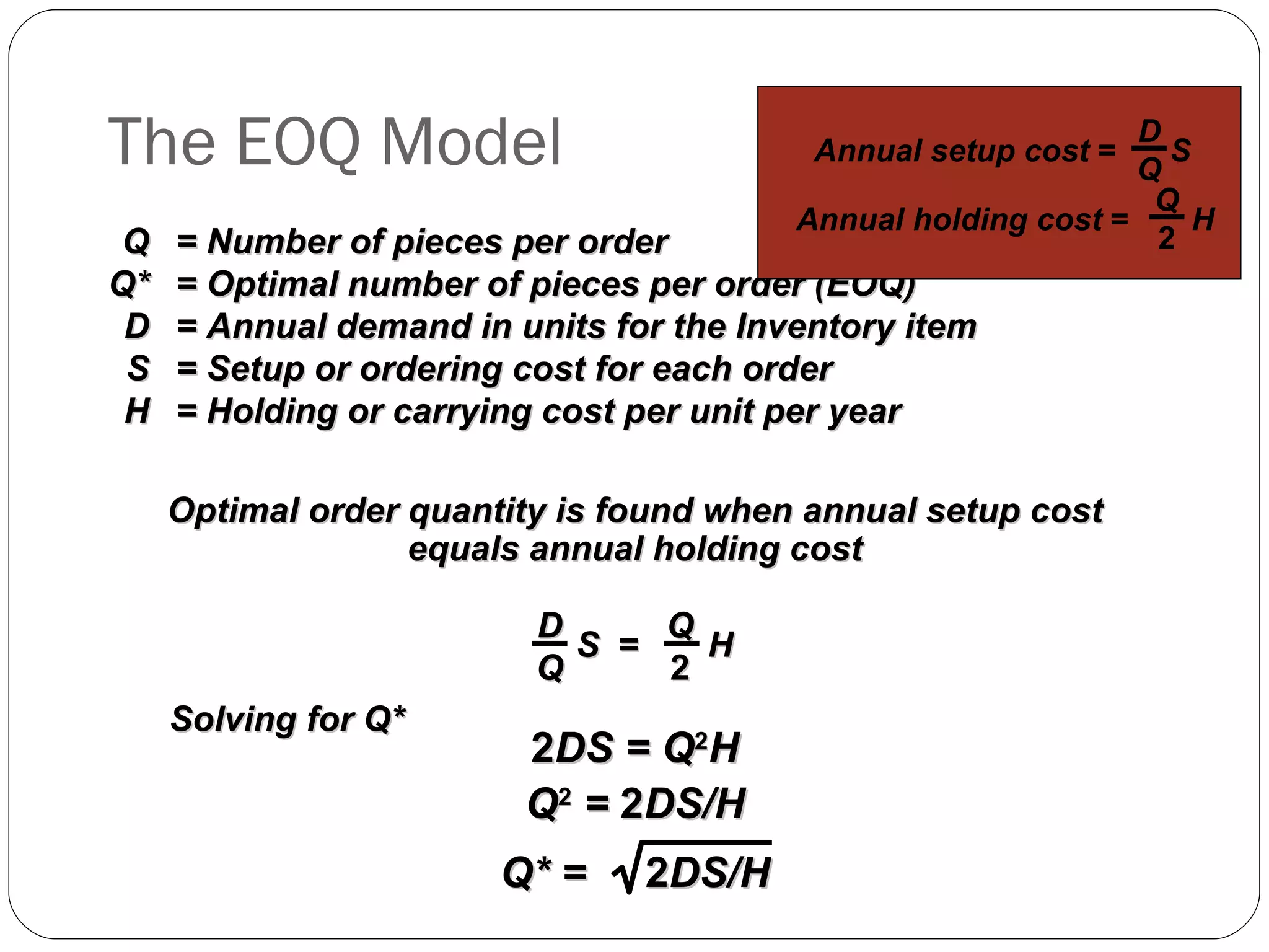
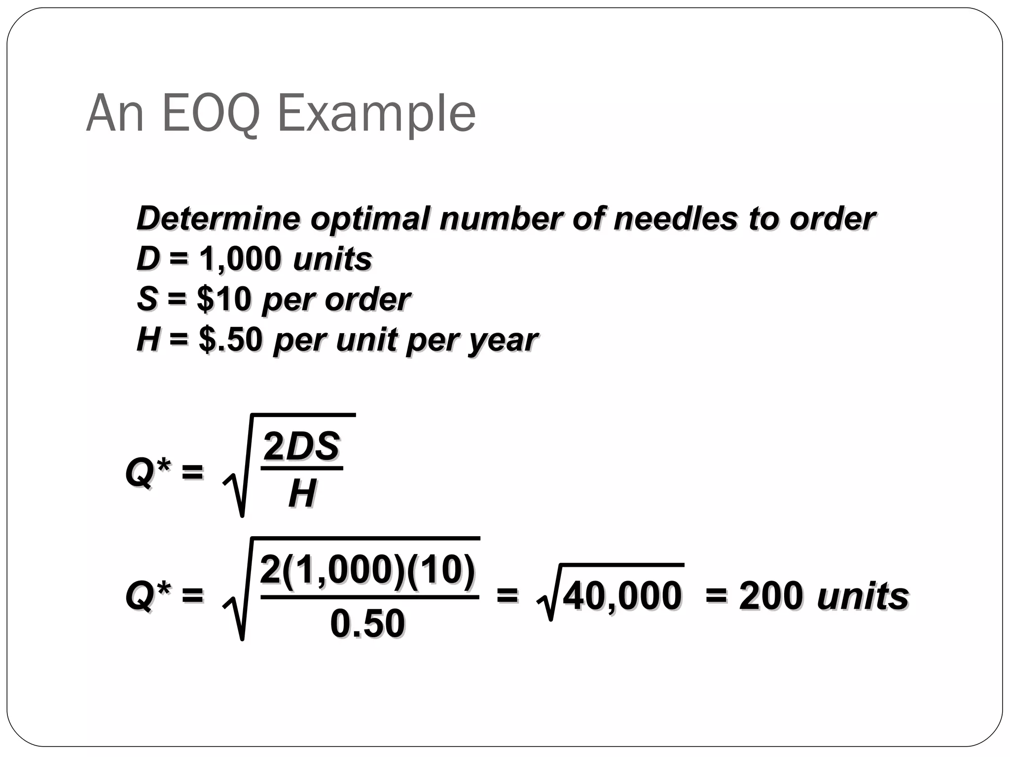
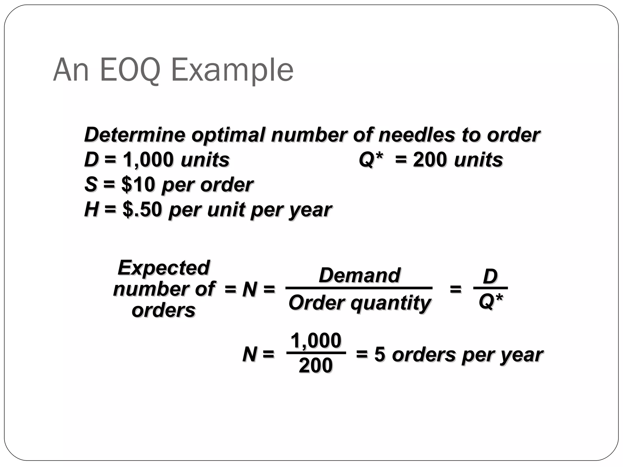
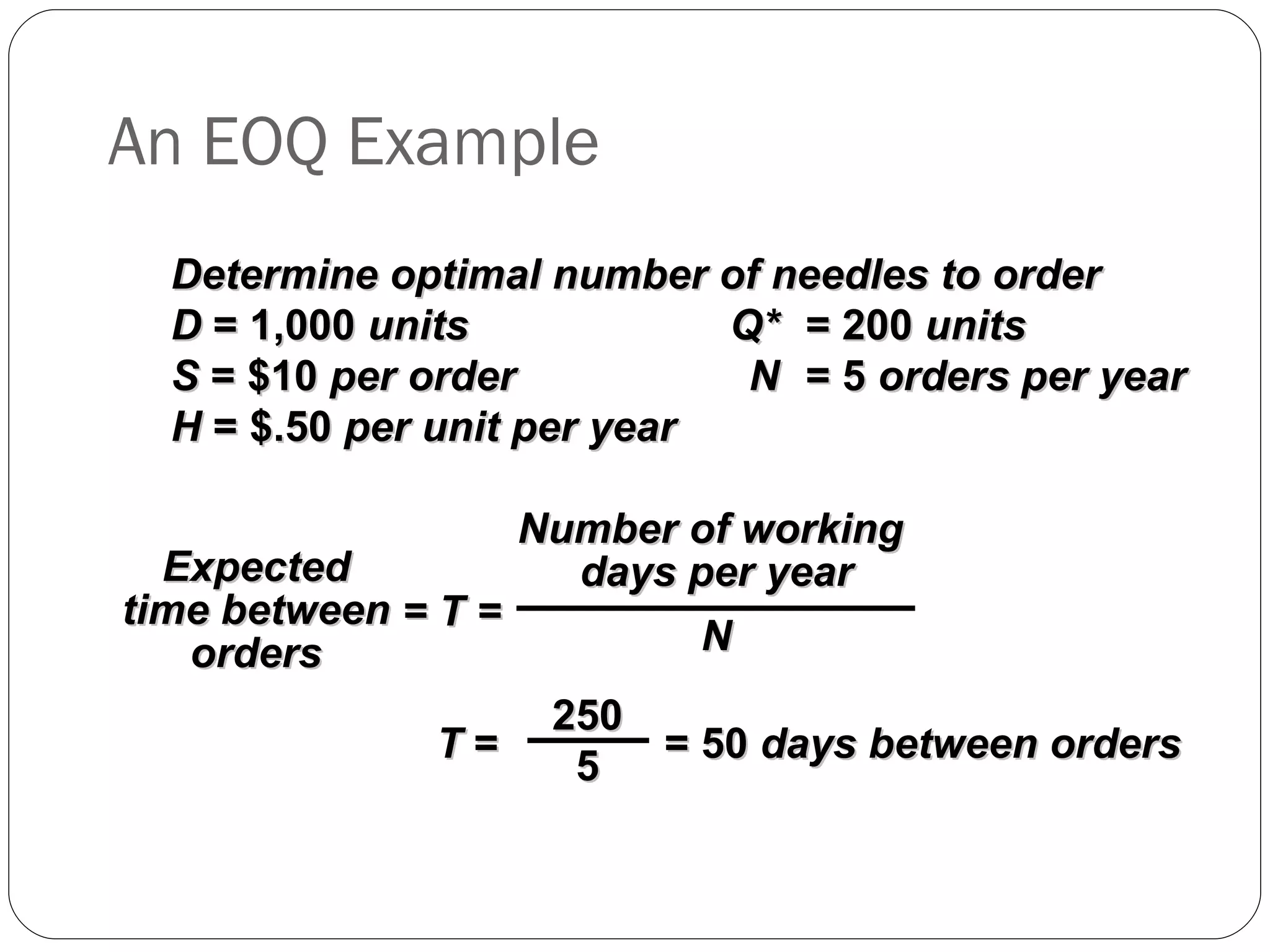
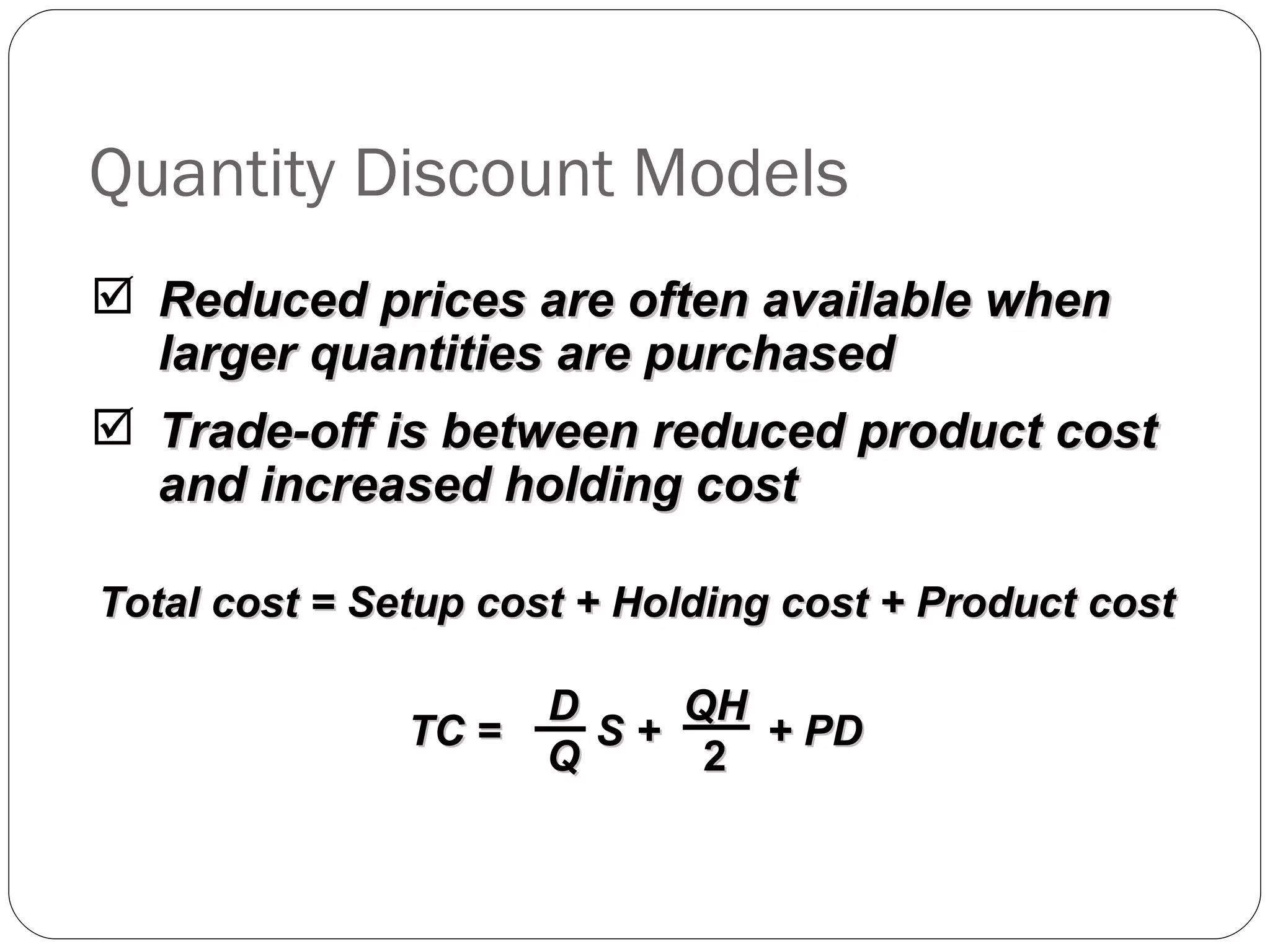
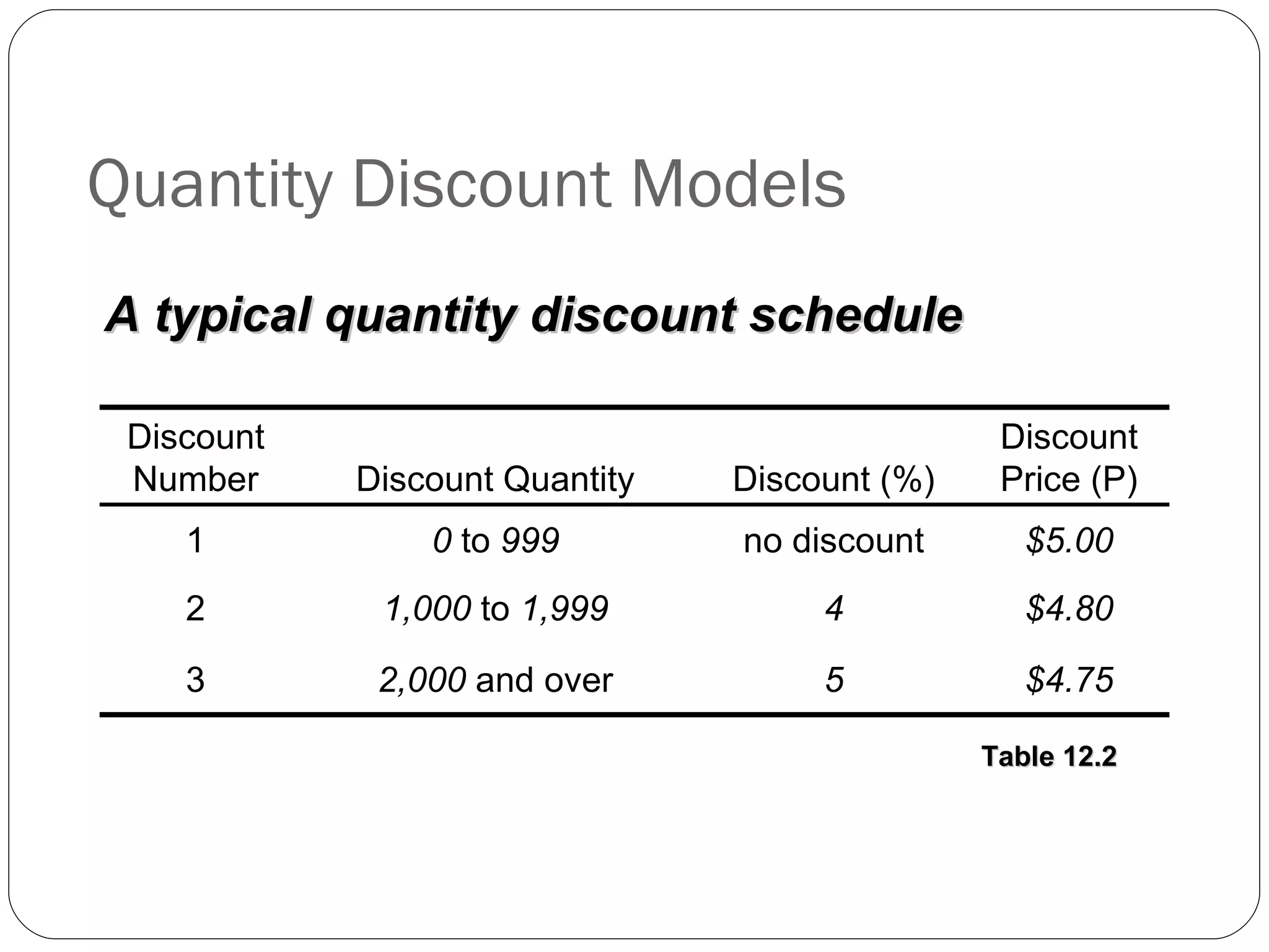
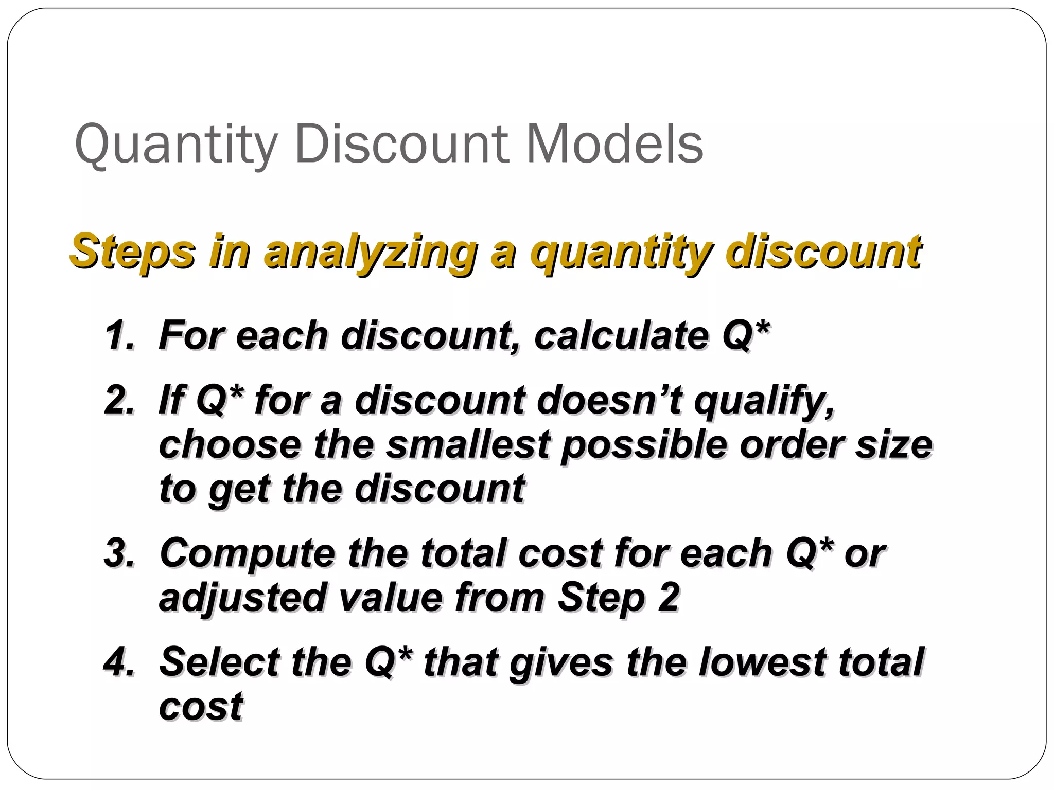
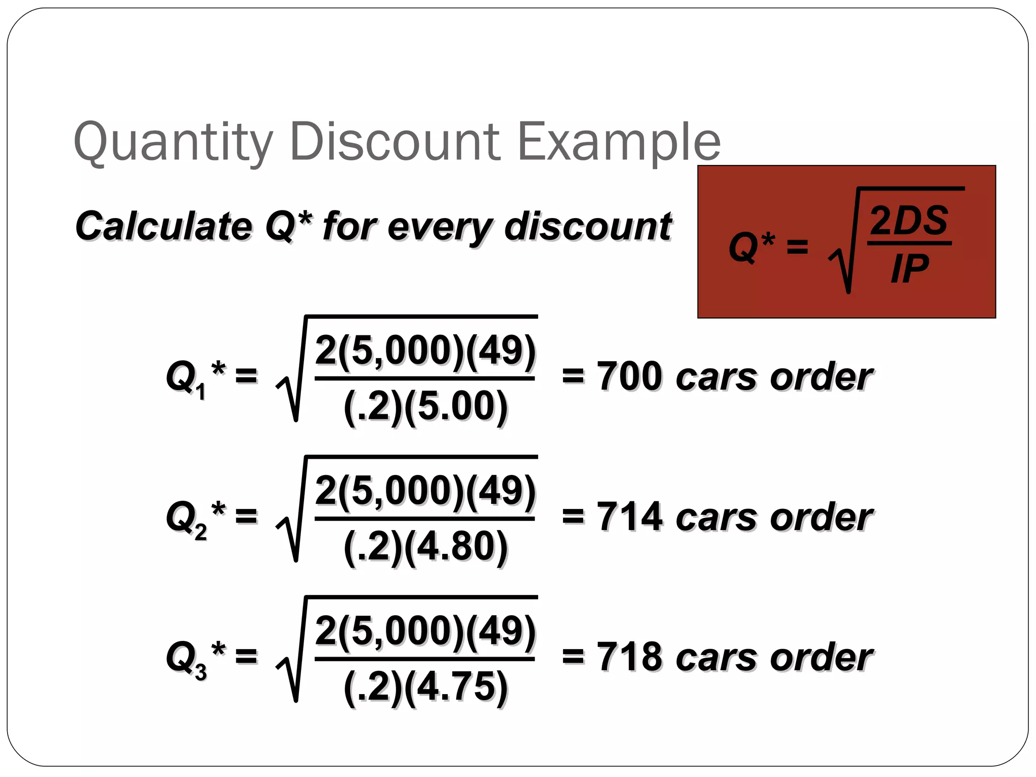
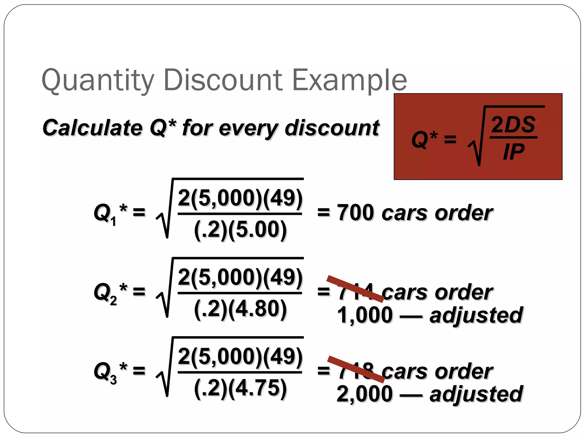
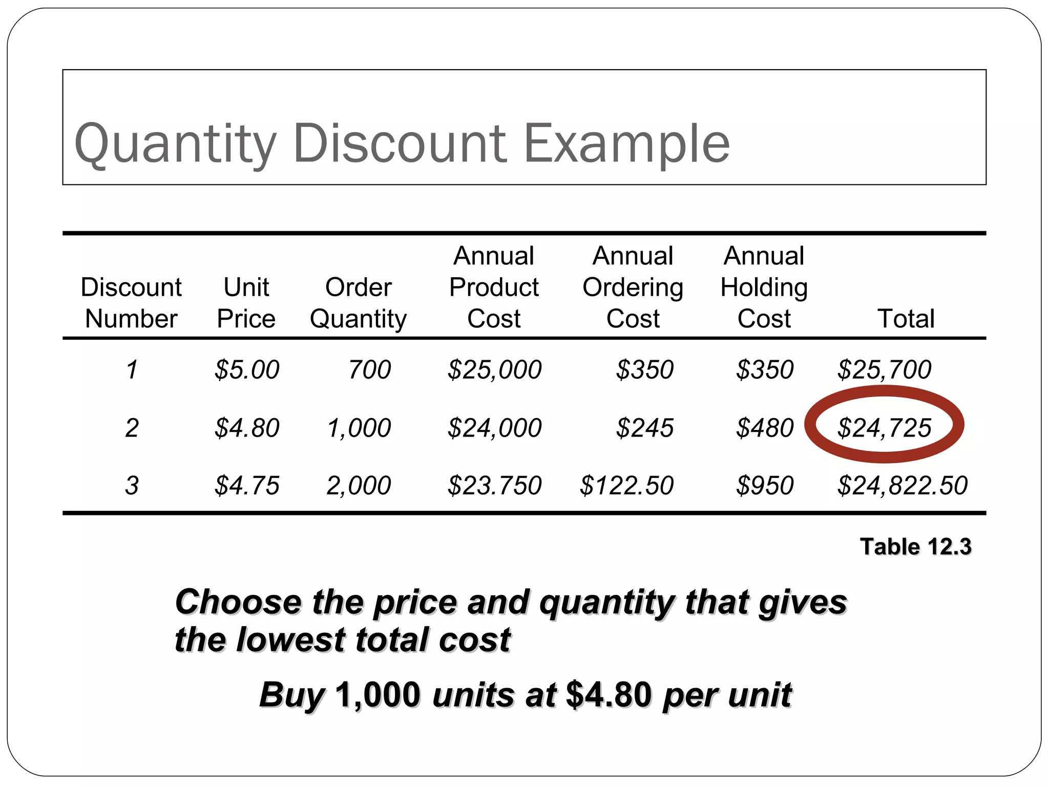
The document discusses inventory management concepts including the economic order quantity (EOQ) model. It provides the assumptions and equations of the EOQ model, which determines the optimal order quantity by minimizing total costs of ordering and holding inventory. It also discusses other inventory models like production order quantity and quantity discounts, as well as inventory classifications like ABC analysis.

1. OPM 533 9- Operations Management Inventory Management Chapter 9

2. Stock of materials Stored capacity Examples What is Inventory? OPM 533 9- © 1995 Corel Corp. © 1984-1994 T/Maker Co. © 1984-1994 T/Maker Co. © 1995 Corel Corp.

3. The Functions of Inventory To ”decouple” or separate various parts of the production process To provide a stock of goods that will provide a “selection” for customers To take advantage of quantity discounts To hedge against inflation and upward price changes OPM 533 9-

4. Types of Inventory Raw material (RM) Work-in-progress (WIP) Maintenance/repair/operating supply (MRO) Finished goods (FG) OPM 533 9-

5. Higher costs Item cost (if purchased) Ordering (or setup) cost Costs of forms, clerks’ wages etc. Holding (or carrying) cost Building lease, insurance, taxes etc. Difficult to control Hides production problems Disadvantages of Inventory OPM 533 9-

6. Inventory Classifications OPM 533 9- Inventory Process stage Demand Type Number & Value Other Raw Material WIP Finished Goods Independent Dependent A Items B Items C Items Maintenance Operating © 1984-1994 T/Maker Co.

7. Run time : Job is at machine and being worked on Setup time : Job is at the work station, and the work station is being "setup." Queue time : Job is where it should be, but is not being processed because other work precedes it. Move time : The time a job spends in transit Wait time : When one process is finished, but the job is waiting to be moved to the next work area. Other: "Just-in-case" inventory. The Material Flow Cycle OPM 533 9- Other Wait Time Move Time Queue Time Setup Time Run Time Input Cycle Time Output

8. Divides on-hand inventory into 3 classes A class, B class, C class Basis is usually annual $ volume $ volume = Annual demand x Unit cost Policies based on ABC analysis Develop class A suppliers more Give tighter physical control of A items Forecast A items more carefully ABC Analysis OPM 533 9-

9. Classifying Items as ABC OPM 533 9- % of Inventory Items 0 20 40 60 80 100 0 50 100 % Annual $ Usage A B C Class % $ Vol % Items A 80 15 B 15 30 C 5 55

10. Physically counting a sample of total inventory on a regular basis Used often with ABC classification A items counted most often (e.g., daily) Cycle Counting OPM 533 9-

11. Advantages of Cycle Counting Eliminates shutdown and interruption of production necessary for annual physical inventories Eliminates annual inventory adjustments Provides trained personnel to audit the accuracy of inventory Allows the cause of errors to be identified and remedial action to be taken Maintains accurate inventory records OPM 533 9-

12. Techniques for Controlling Service Inventory Include: Good personnel selection, training, and discipline Tight control of incoming shipments Effective control of all goods leaving the facility OPM 533 9-

13. Independent versus Dependent Demand Independent demand - demand for item is independent of demand for any other item Dependent demand - demand for item is dependent upon the demand for some other item OPM 533 9-

14. Inventory Costs Holding costs - associated with holding or “carrying” inventory over time; e.g. obsolescence, insurance, extra staffing, interest, pilferage, damage, warehousing, etc. Ordering costs - associated with costs of placing order and receiving goods; eg. Supplies, forms, order processing, clerical support, etc. Setup costs - cost to prepare a machine or process for manufacturing an order; e.g. clean-up costs, re-tooling costs, adjustment costs, etc. OPM 533 9-

15. Inventory Holding Costs (Approximate Ranges) Category Housing costs (building rent, depreciation, operating cost, taxes, insurance) Material handling costs (equipment, lease or depreciation, power, operating cost) Labor cost from extra handling Investment costs (borrowing costs, taxes, and insurance on inventory) Pilferage, scrap, and obsolescence Overall carrying cost Cost as a % of Inventory Value 6% (3 - 10%) 3% (1 - 3.5%) 3% (3 - 5%) 11% (6 - 24%) 3% (2 - 5%) 26% OPM 533 9-

16. Fixed order-quantity models Economic order quantity Production order quantity Quantity discount Probabilistic models Fixed order-period models Inventory Models OPM 533 9- Help answer the inventory planning questions! © 1984-1994 T/Maker Co.

17. Known and constant demand Known and constant lead time Instantaneous receipt of material No quantity discounts Only order (setup) cost and holding cost No stockouts 1. EOQ Assumptions OPM 533 9-

18. Inventory Usage Over Time OPM 533 9- Time Inventory Level Average Inventory (Q*/2) 0 Minimum inventory Order quantity = Q (maximum inventory level) Usage Rate

19. EOQ Model How Much to Order? OPM 533 9- Order quantity Annual Cost Holding Cost Curve Total Cost Curve Order (Setup) Cost Curve Optimal Order Quantity (Q*) Minimum total cost

20. More units must be stored if more are ordered Why Holding Costs Increase OPM 533 9- Purchase Order Description Qty. Microwave 1 Order quantity Purchase Order Description Qty. Microwave 1000 Order quantity

21. Cost is spread over more units Example: You need 1000 microwave ovens Why Order Costs Decrease OPM 533 9- Purchase Order Description Qty. Microwave 1 Purchase Order Description Qty. Microwave 1 Purchase Order Description Qty. Microwave 1 Purchase Order Description Qty. Microwave 1 1 Order (Postage $ 0.33) 1000 Orders (Postage $330) Order quantity Purchase Order Description Qty . Microwave 1000

22. Deriving an EOQ Develop an expression for setup or ordering costs Develop an expression for holding cost Set setup cost equal to holding cost Solve the resulting equation for the best order quantity OPM 533 9-

23. EOQ Model Equations OPM 533 9- Optimal Order Quantity Expected Number of Orders Expected Time Between Orders Working Days / Year Working Days / Year = = × × = = = = = = × Q* D S H N D Q * T N d D ROP d L 2 D = Demand per year S = Setup (order) cost per order H = Holding (carrying) cost d = Demand per day L = Lead time in days

24. The Reorder Point (ROP) Curve OPM 533 9- Q* ROP (Units) Slope = units/day = d Lead time = L Time (days) Inventory level (units)

25. Answers how much to order and when to order Allows partial receipt of material Other EOQ assumptions apply Suited for production environment Material produced, used immediately Provides production lot size Lower holding cost than EOQ model 2. Production Order Quantity Model OPM 533 9-

26. Reasons for Variability in Production Most variability is caused by waste or by poor management. Specific causes include: employees, machines, and suppliers produce units that do not conform to standards, are late or are not the proper quantity inaccurate engineering drawings or specifications production personnel try to produce before drawings or specifications are complete customer demands are unknown OPM 533 9-

27. POQ Model Equations OPM 533 9- D = Demand per year S = Setup cost H = Holding cost d = Demand per day p = Production per day Optimal Order Quantity Setup Cost Holding Cost = = - = * = * = Q H* d p Q D Q S p * 1 ( 0.5 * H * Q - d p 1 ) 1 ( ) 2*D*S ( ) Maximum inventory level - d p

28. Answers how much to order & when to order Allows quantity discounts Reduced price when item is purchased in larger quantities Other EOQ assumptions apply Trade-off is between lower price & increased holding cost 3. Quantity Discount Model OPM 533 9-

29. Inventory Usage Over Time Figure 12.3 Order quantity = Q (maximum inventory level) Inventory level Time Usage rate Average inventory on hand Q 2 Minimum inventory

30. Minimizing Costs Objective is to minimize total costs Table 11.5 Annual cost Order quantity Curve for total cost of holding and setup Holding cost curve Setup (or order) cost curve Minimum total cost Optimal order quantity

31. The EOQ Model Q = Number of pieces per order Q* = Optimal number of pieces per order (EOQ) D = Annual demand in units for the Inventory item S = Setup or ordering cost for each order H = Holding or carrying cost per unit per year Annual setup cost = ( Number of orders placed per year ) x ( Setup or order cost per order ) Annual demand Number of units in each order Setup or order cost per order = = ( S ) D Q Annual setup cost = S D Q

32. The EOQ Model Q = Number of pieces per order Q* = Optimal number of pieces per order (EOQ) D = Annual demand in units for the Inventory item S = Setup or ordering cost for each order H = Holding or carrying cost per unit per year Annual holding cost = ( Average inventory level ) x ( Holding cost per unit per year ) Order quantity 2 = ( Holding cost per unit per year ) = ( H ) Q 2 Annual setup cost = S D Q Annual holding cost = H Q 2

33. The EOQ Model Q = Number of pieces per order Q* = Optimal number of pieces per order (EOQ) D = Annual demand in units for the Inventory item S = Setup or ordering cost for each order H = Holding or carrying cost per unit per year Optimal order quantity is found when annual setup cost equals annual holding cost Solving for Q* Annual setup cost = S D Q Annual holding cost = H Q 2 D Q S = H Q 2 2 DS = Q 2 H Q 2 = 2 DS/H Q* = 2 DS/H

34. An EOQ Example Determine optimal number of needles to order D = 1,000 units S = $10 per order H = $.50 per unit per year Q* = 2 DS H Q* = 2(1,000)(10) 0.50 = 40,000 = 200 units

35. An EOQ Example Determine optimal number of needles to order D = 1,000 units Q* = 200 units S = $10 per order H = $.50 per unit per year = N = = Expected number of orders Demand Order quantity D Q* N = = 5 orders per year 1,000 200

36. An EOQ Example Determine optimal number of needles to order D = 1,000 units Q* = 200 units S = $10 per order N = 5 orders per year H = $.50 per unit per year = T = Expected time between orders Number of working days per year N T = = 50 days between orders 250 5

37. An EOQ Example Determine optimal number of needles to order D = 1,000 units Q* = 200 units S = $10 per order N = 5 orders per year H = $.50 per unit per year T = 50 days Total annual cost = Setup cost + Holding cost TC = (5)($10) + (100)($.50) = $50 + $50 = $100 TC = S + H D Q Q 2 TC = ($10) + ($.50) 1,000 200 200 2

38. An EOQ Example with safety stock Determine optimal number of needles to order D = 1,000 units Q* = 200 units S = $10 per order N = 5 orders per year H = $.50 per unit per year T = 50 days Safety Stock (ss) = 10 units Total annual cost = Setup cost + Holding cost TC = (5)($10) + (200)($.50) = $50 + $100 = $150 TC = S + ( + ss ) H D Q Q 2 TC = ($10) + (100 + )($.50) 1,000 200 200 2

39. Reorder Points EOQ answers the “how much” question The reorder point (ROP) tells when to order = d x L ROP = Lead time for a new order in days Demand per day d = D Number of working days in a year

40. Reorder Point Curve Figure 12.5 Q* ROP (units) Inventory level (units) Time (days) Lead time = L Slope = units/day = d

41. Reorder Point Example Demand = 8,000 DVDs per year 250 working day year Lead time for orders is 3 working days ROP = d x L = 8,000/250 = 32 units = 32 units per day x 3 days = 96 units d = D Number of working days in a year

42. Reorder point with Safety Stock Annual Demand = 25,000 units Number of working days in a year 250 days Lead time = 5 days Safety stock (ss) = 2 days usage ROP = d x l + ss d= D / Number of days work in a year d= 25,000 / 250 = 100 units ss= 2 days x 100 = 200 ROP = 100 x 5 + 200 = 700 units

43. Quantity Discount Models Reduced prices are often available when larger quantities are purchased Trade-off is between reduced product cost and increased holding cost Total cost = Setup cost + Holding cost + Product cost TC = S + + PD D Q QH 2

44. Quantity Discount Models Table 12.2 A typical quantity discount schedule Discount Number Discount Quantity Discount (%) Discount Price (P) 1 0 to 999 no discount $5.00 2 1,000 to 1,999 4 $4.80 3 2,000 and over 5 $4.75

45. Quantity Discount Models For each discount, calculate Q* If Q* for a discount doesn’t qualify, choose the smallest possible order size to get the discount Compute the total cost for each Q* or adjusted value from Step 2 Select the Q* that gives the lowest total cost Steps in analyzing a quantity discount

46. Quantity Discount Models Figure 12.7 1,000 2,000 Total cost $ 0 Order quantity Q* for discount 2 is below the allowable range at point a and must be adjusted upward to 1,000 units at point b a b 1st price break 2nd price break Total cost curve for discount 1 Total cost curve for discount 2 Total cost curve for discount 3

47. Quantity Discount Example Calculate Q* for every discount Q* = 2 DS IP Q 1 * = = 700 cars order 2(5,000)(49) (.2)(5.00) Q 2 * = = 714 cars order 2(5,000)(49) (.2)(4.80) Q 3 * = = 718 cars order 2(5,000)(49) (.2)(4.75)

48. Quantity Discount Example Calculate Q* for every discount Q* = 2 DS IP Q 1 * = = 700 cars order 2(5,000)(49) (.2)(5.00) Q 2 * = = 714 cars order 2(5,000)(49) (.2)(4.80) Q 3 * = = 718 cars order 2(5,000)(49) (.2)(4.75) 1,000 — adjusted 2,000 — adjusted

49. Quantity Discount Example Table 12.3 Choose the price and quantity that gives the lowest total cost Buy 1,000 units at $4.80 per unit Discount Number Unit Price Order Quantity Annual Product Cost Annual Ordering Cost Annual Holding Cost Total 1 $5.00 700 $25,000 $350 $350 $25,700 2 $4.80 1,000 $24,000 $245 $480 $24,725 3 $4.75 2,000 $23.750 $122.50 $950 $24,822.50