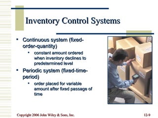
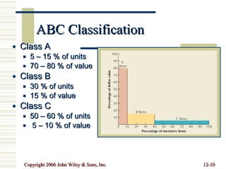
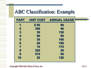
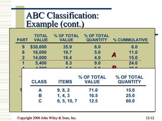
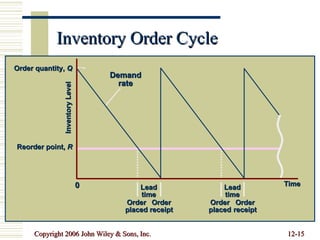
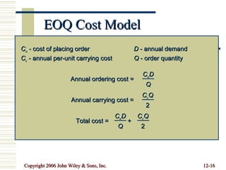
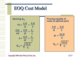
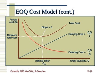
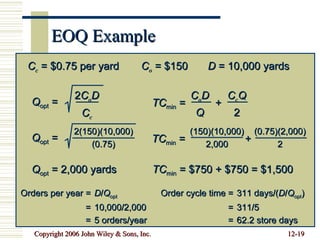
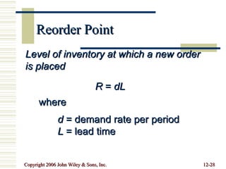
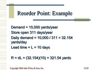
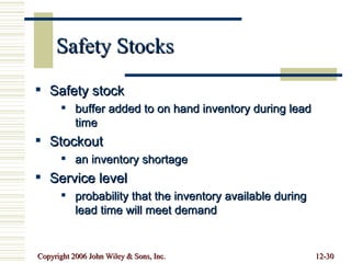
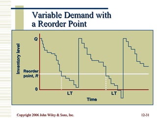
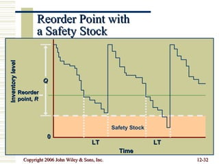
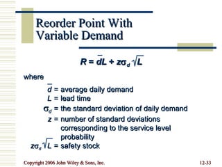
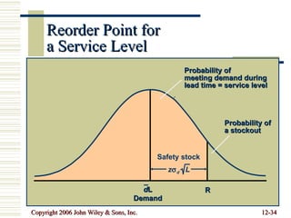
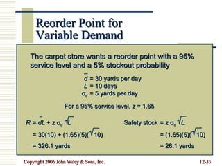
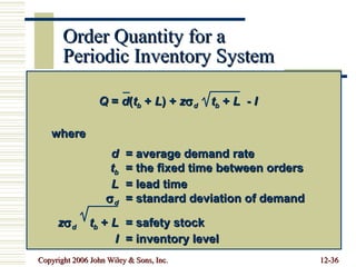
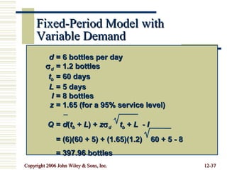
Beni Asllani University of Tennessee at Chattanooga Inventory Management Operations Management - 5 th  Edition Chapter 12 Roberta Russell & Bernard W. Taylor, III
Lecture Outline Elements of Inventory Management Inventory Control Systems Economic Order Quantity Models Quantity Discounts Reorder Point Order Quantity for a Periodic Inventory System
What Is Inventory? Stock of items kept to meet future demand Purpose of inventory management how many units to order when to order
Types of Inventory Raw materials Purchased parts and supplies Work-in-process (partially completed) products (WIP) Items being transported Tools and equipment
Inventory and Supply Chain Management Bullwhip effect demand information is distorted as it moves away from the end-use customer higher safety stock inventories to are stored to compensate Seasonal or cyclical demand Inventory provides independence from vendors Take advantage of price discounts Inventory provides independence between stages and avoids work stop-pages
Two Forms of Demand Dependent Demand for items used to produce final products  Tires stored at a Goodyear plant are an example of a dependent demand item Independent Demand for items used by external customers Cars, appliances, computers, and houses are examples of independent demand inventory
Inventory and Quality Management Customers usually perceive quality service as availability of goods they want when they want them Inventory must be sufficient to provide high-quality customer service in TQM
Inventory Costs Carrying cost cost of  holding an item in inventory Ordering cost cost of  replenishing inventory Shortage cost temporary or permanent loss of sales when demand cannot be met
Inventory Control Systems Continuous system (fixed-order-quantity) constant amount ordered when inventory declines to predetermined level Periodic system (fixed-time-period) order placed for variable amount after fixed passage of time
ABC Classification Class A 5 – 15 % of units 70 – 80 % of value  Class B 30 % of units 15 % of value Class C 50 – 60 % of units 5 – 10 % of value
ABC Classification: Example 1 $ 60 90 2 350 40 3 30 130 4 80 60 5 30 100 6 20 180 7 10 170 8 320 50 9 510 60 10 20 120 PART UNIT COST ANNUAL USAGE
ABC Classification: Example (cont.) Example 10.1 1 $ 60 90 2 350 40 3 30 130 4 80 60 5 30 100 6 20 180 7 10 170 8 320 50 9 510 60 10 20 120 PART UNIT COST ANNUAL USAGE TOTAL % OF TOTAL % OF TOTAL PART VALUE VALUE QUANTITY % CUMMULATIVE 9 $30,600 35.9 6.0 6.0 8 16,000 18.7 5.0 11.0 2 14,000 16.4 4.0 15.0 1 5,400 6.3 9.0 24.0 4 4,800 5.6 6.0 30.0 3 3,900 4.6 10.0 40.0 6 3,600 4.2 18.0 58.0 5 3,000 3.5 13.0 71.0 10 2,400 2.8 12.0 83.0 7 1,700 2.0 17.0 100.0 $85,400 A B C % OF TOTAL % OF TOTAL CLASS ITEMS VALUE QUANTITY A 9, 8, 2 71.0 15.0 B 1, 4, 3 16.5 25.0 C 6, 5, 10, 7 12.5 60.0
Economic Order Quantity (EOQ) Models EOQ optimal order quantity that will minimize total inventory costs Basic EOQ model Production quantity model
Assumptions of Basic EOQ Model Demand is known with certainty and is constant over time No shortages are allowed Lead time for the receipt of orders is constant Order quantity is received all at once
Inventory Order Cycle Demand rate Time Lead time Lead time Order placed Order placed Order receipt Order receipt Inventory Level Reorder point,  R Order quantity,  Q 0
EOQ Cost Model C o  - cost of placing order D  - annual demand C c  - annual per-unit carrying cost Q  - order quantity Annual ordering cost = C o D Q Annual carrying cost = C c Q 2 Total cost =  + C o D Q C c Q 2
EOQ Cost Model TC =  + C o D Q C c Q 2 =  + C o D Q 2 C c 2  TC  Q 0 =  + C 0 D Q 2 C c 2 Q opt  = 2 C o D C c Deriving  Q opt Proving equality of costs at optimal point = C o D Q C c Q 2 Q 2   = 2 C o D C c Q opt  = 2 C o D C c
EOQ Cost Model (cont.) Order Quantity,  Q Annual cost ($) Total Cost Carrying Cost = C c Q 2 Slope = 0 Minimum total cost Optimal order Q opt Ordering Cost = C o D Q
EOQ Example Orders per year = D / Q opt = 10,000/2,000 = 5 orders/year Order cycle time = 311 days/( D / Q opt ) = 311/5 = 62.2 store days C c  = $0.75 per yard C o  = $150 D  = 10,000 yards Q opt  = 2 C o D C c Q opt  = 2(150)(10,000) (0.75) Q opt  = 2,000 yards TC min  =  + C o D Q C c Q 2 TC min  =  + (150)(10,000) 2,000 (0.75)(2,000) 2 TC min  = $750 + $750 = $1,500
Production Quantity Model An inventory system in which an order is received gradually, as inventory is simultaneously being depleted AKA non-instantaneous receipt model assumption that  Q  is received all at once is relaxed p -  daily rate at which an order is received over time, a.k.a.  production rate d -  daily rate at which inventory is demanded
Production Quantity Model (cont.) Q (1- d/p ) Inventory level (1- d/p ) Q 2 Time 0 Order receipt period Begin order receipt End order receipt Maximum inventory level Average inventory level
Production Quantity Model (cont.) p  = production rate d  = demand rate Maximum inventory level = Q  -  d = Q  1 - Q p d p Average inventory level =  1 - Q 2 d p TC  =  +  1 - d p C o D Q C c Q 2 Q opt  = 2 C o D C c   1 -  d p
Production Quantity Model: Example C c  = $0.75 per yard C o  = $150 D  = 10,000 yards d  = 10,000/311 = 32.2 yards per day p  = 150 yards per day Q opt  =  =  = 2,256.8 yards 2 C o D C c   1 -  d p 2(150)(10,000) 0.75  1 -  32.2 150 TC  =  +  1 -  = $1,329 d p C o D Q C c Q 2 Production run =  =  = 15.05 days per order Q p 2,256.8 150
Production Quantity Model: Example (cont.) Number of production runs =  =  = 4.43 runs/year D Q 10,000 2,256.8 Maximum inventory level = Q  1 -  = 2,256.8  1 - = 1,772 yards d p 32.2 150
Quantity Discounts Price per unit decreases as order quantity increases TC  =  +  +  PD C o D Q C c Q 2 where P  = per unit price of the item D  = annual demand
Quantity Discount Model (cont.) Q opt Carrying cost  Ordering cost  Inventory cost ($) Q ( d 1  ) = 100 Q ( d 2  ) = 200 TC  ( d 2  = $6 )  TC  ( d 1  = $8 )   TC  = ($10 )   ORDER SIZE  PRICE 0 - 99   $10 100 – 199  8 ( d 1 ) 200+  6 ( d 2 )
Quantity Discount: Example C o  = $2,500  C c  = $190 per computer  D  = 200 QUANTITY PRICE 1 - 49 $1,400 50 - 89 1,100 90+ 900 Q opt  =  =  = 72.5 PCs 2 C o D C c 2(2500)(200) 190 TC  =  +  +  PD  = $233,784  C o D Q opt C c Q opt 2 For  Q  = 72.5 TC  =  +  +  PD  = $194,105 C o D Q C c Q 2 For  Q  = 90
Reorder Point Level of inventory at which a new order is placed  R  =  dL where d  = demand rate per period L  = lead time
Reorder Point: Example Demand = 10,000 yards/year Store open 311 days/year Daily demand = 10,000 / 311 = 32.154 yards/day Lead time = L = 10 days R = dL = (32.154)(10) = 321.54 yards
Safety Stocks  Safety stock buffer added to on hand inventory during lead time Stockout  an inventory shortage Service level  probability that the inventory available during lead time will meet demand
Variable Demand with  a Reorder Point Reorder point,  R Q LT Time LT Inventory level 0
Reorder Point with  a Safety Stock Reorder point,  R Q LT Time LT Inventory level 0 Safety Stock
Reorder Point With  Variable Demand R  =  dL  +  z  d   L where d = average daily demand L = lead time  d = the standard deviation of daily demand  z = number of standard deviations corresponding to the service level probability z  d   L = safety stock
Reorder Point for  a Service Level Probability of  meeting demand during  lead time = service level Probability of  a stockout R Safety stock d L Demand z  d   L
Reorder Point for  Variable Demand The carpet store wants a reorder point with a 95% service level and a 5% stockout probability For a 95% service level,  z  = 1.65 d = 30 yards per day L = 10 days  d = 5 yards per day R =  dL  +  z    d   L = 30(10) + (1.65)(5)(  10) = 326.1 yards Safety stock =  z    d   L = (1.65)(5)(  10) = 26.1 yards
Order Quantity for a  Periodic Inventory System Q  =  d ( t b  +  L ) +  z  d   t b  +  L   -  I where d = average demand rate t b = the fixed time between orders L = lead time  d = standard deviation of demand   z  d   t b  +  L = safety stock I = inventory level
Fixed-Period Model with Variable Demand d = 6 bottles per day  d = 1.2 bottles t b = 60 days L = 5 days I = 8 bottles z = 1.65 (for a 95% service level) Q =  d ( t b  +  L ) +  z  d   t b  +  L   -  I = (6)(60 + 5) + (1.65)(1.2)  60 + 5 - 8 = 397.96 bottles
Copyright 2006 John Wiley & Sons, Inc. All rights reserved.  Reproduction or translation of this work beyond that permitted in section 117 of the 1976 United States Copyright Act without express permission of the copyright owner is unlawful.  Request for further information should be addressed to the Permission Department, John Wiley & Sons, Inc.  The purchaser may make back-up copies for his/her own use only and not for distribution or resale.  The Publisher assumes no responsibility for errors, omissions, or damages caused by the use of these programs or from the use of the information herein.

Inventory Man2

  • 1.
    Beni Asllani Universityof Tennessee at Chattanooga Inventory Management Operations Management - 5 th Edition Chapter 12 Roberta Russell & Bernard W. Taylor, III
  • 2.
    Lecture Outline Elementsof Inventory Management Inventory Control Systems Economic Order Quantity Models Quantity Discounts Reorder Point Order Quantity for a Periodic Inventory System
  • 3.
    What Is Inventory?Stock of items kept to meet future demand Purpose of inventory management how many units to order when to order
  • 4.
    Types of InventoryRaw materials Purchased parts and supplies Work-in-process (partially completed) products (WIP) Items being transported Tools and equipment
  • 5.
    Inventory and SupplyChain Management Bullwhip effect demand information is distorted as it moves away from the end-use customer higher safety stock inventories to are stored to compensate Seasonal or cyclical demand Inventory provides independence from vendors Take advantage of price discounts Inventory provides independence between stages and avoids work stop-pages
  • 6.
    Two Forms ofDemand Dependent Demand for items used to produce final products Tires stored at a Goodyear plant are an example of a dependent demand item Independent Demand for items used by external customers Cars, appliances, computers, and houses are examples of independent demand inventory
  • 7.
    Inventory and QualityManagement Customers usually perceive quality service as availability of goods they want when they want them Inventory must be sufficient to provide high-quality customer service in TQM
  • 8.
    Inventory Costs Carryingcost cost of holding an item in inventory Ordering cost cost of replenishing inventory Shortage cost temporary or permanent loss of sales when demand cannot be met
  • 9.
    Inventory Control SystemsContinuous system (fixed-order-quantity) constant amount ordered when inventory declines to predetermined level Periodic system (fixed-time-period) order placed for variable amount after fixed passage of time
  • 10.
    ABC Classification ClassA 5 – 15 % of units 70 – 80 % of value Class B 30 % of units 15 % of value Class C 50 – 60 % of units 5 – 10 % of value
  • 11.
    ABC Classification: Example1 $ 60 90 2 350 40 3 30 130 4 80 60 5 30 100 6 20 180 7 10 170 8 320 50 9 510 60 10 20 120 PART UNIT COST ANNUAL USAGE
  • 12.
    ABC Classification: Example(cont.) Example 10.1 1 $ 60 90 2 350 40 3 30 130 4 80 60 5 30 100 6 20 180 7 10 170 8 320 50 9 510 60 10 20 120 PART UNIT COST ANNUAL USAGE TOTAL % OF TOTAL % OF TOTAL PART VALUE VALUE QUANTITY % CUMMULATIVE 9 $30,600 35.9 6.0 6.0 8 16,000 18.7 5.0 11.0 2 14,000 16.4 4.0 15.0 1 5,400 6.3 9.0 24.0 4 4,800 5.6 6.0 30.0 3 3,900 4.6 10.0 40.0 6 3,600 4.2 18.0 58.0 5 3,000 3.5 13.0 71.0 10 2,400 2.8 12.0 83.0 7 1,700 2.0 17.0 100.0 $85,400 A B C % OF TOTAL % OF TOTAL CLASS ITEMS VALUE QUANTITY A 9, 8, 2 71.0 15.0 B 1, 4, 3 16.5 25.0 C 6, 5, 10, 7 12.5 60.0
  • 13.
    Economic Order Quantity(EOQ) Models EOQ optimal order quantity that will minimize total inventory costs Basic EOQ model Production quantity model
  • 14.
    Assumptions of BasicEOQ Model Demand is known with certainty and is constant over time No shortages are allowed Lead time for the receipt of orders is constant Order quantity is received all at once
  • 15.
    Inventory Order CycleDemand rate Time Lead time Lead time Order placed Order placed Order receipt Order receipt Inventory Level Reorder point, R Order quantity, Q 0
  • 16.
    EOQ Cost ModelC o - cost of placing order D - annual demand C c - annual per-unit carrying cost Q - order quantity Annual ordering cost = C o D Q Annual carrying cost = C c Q 2 Total cost = + C o D Q C c Q 2
  • 17.
    EOQ Cost ModelTC = + C o D Q C c Q 2 = + C o D Q 2 C c 2  TC  Q 0 = + C 0 D Q 2 C c 2 Q opt = 2 C o D C c Deriving Q opt Proving equality of costs at optimal point = C o D Q C c Q 2 Q 2 = 2 C o D C c Q opt = 2 C o D C c
  • 18.
    EOQ Cost Model(cont.) Order Quantity, Q Annual cost ($) Total Cost Carrying Cost = C c Q 2 Slope = 0 Minimum total cost Optimal order Q opt Ordering Cost = C o D Q
  • 19.
    EOQ Example Ordersper year = D / Q opt = 10,000/2,000 = 5 orders/year Order cycle time = 311 days/( D / Q opt ) = 311/5 = 62.2 store days C c = $0.75 per yard C o = $150 D = 10,000 yards Q opt = 2 C o D C c Q opt = 2(150)(10,000) (0.75) Q opt = 2,000 yards TC min = + C o D Q C c Q 2 TC min = + (150)(10,000) 2,000 (0.75)(2,000) 2 TC min = $750 + $750 = $1,500
  • 20.
    Production Quantity ModelAn inventory system in which an order is received gradually, as inventory is simultaneously being depleted AKA non-instantaneous receipt model assumption that Q is received all at once is relaxed p - daily rate at which an order is received over time, a.k.a. production rate d - daily rate at which inventory is demanded
  • 21.
    Production Quantity Model(cont.) Q (1- d/p ) Inventory level (1- d/p ) Q 2 Time 0 Order receipt period Begin order receipt End order receipt Maximum inventory level Average inventory level
  • 22.
    Production Quantity Model(cont.) p = production rate d = demand rate Maximum inventory level = Q - d = Q 1 - Q p d p Average inventory level = 1 - Q 2 d p TC = + 1 - d p C o D Q C c Q 2 Q opt = 2 C o D C c 1 - d p
  • 23.
    Production Quantity Model:Example C c = $0.75 per yard C o = $150 D = 10,000 yards d = 10,000/311 = 32.2 yards per day p = 150 yards per day Q opt = = = 2,256.8 yards 2 C o D C c 1 - d p 2(150)(10,000) 0.75 1 - 32.2 150 TC = + 1 - = $1,329 d p C o D Q C c Q 2 Production run = = = 15.05 days per order Q p 2,256.8 150
  • 24.
    Production Quantity Model:Example (cont.) Number of production runs = = = 4.43 runs/year D Q 10,000 2,256.8 Maximum inventory level = Q 1 - = 2,256.8 1 - = 1,772 yards d p 32.2 150
  • 25.
    Quantity Discounts Priceper unit decreases as order quantity increases TC = + + PD C o D Q C c Q 2 where P = per unit price of the item D = annual demand
  • 26.
    Quantity Discount Model(cont.) Q opt Carrying cost Ordering cost Inventory cost ($) Q ( d 1 ) = 100 Q ( d 2 ) = 200 TC ( d 2 = $6 ) TC ( d 1 = $8 ) TC = ($10 ) ORDER SIZE PRICE 0 - 99 $10 100 – 199 8 ( d 1 ) 200+ 6 ( d 2 )
  • 27.
    Quantity Discount: ExampleC o = $2,500 C c = $190 per computer D = 200 QUANTITY PRICE 1 - 49 $1,400 50 - 89 1,100 90+ 900 Q opt = = = 72.5 PCs 2 C o D C c 2(2500)(200) 190 TC = + + PD = $233,784 C o D Q opt C c Q opt 2 For Q = 72.5 TC = + + PD = $194,105 C o D Q C c Q 2 For Q = 90
  • 28.
    Reorder Point Levelof inventory at which a new order is placed R = dL where d = demand rate per period L = lead time
  • 29.
    Reorder Point: ExampleDemand = 10,000 yards/year Store open 311 days/year Daily demand = 10,000 / 311 = 32.154 yards/day Lead time = L = 10 days R = dL = (32.154)(10) = 321.54 yards
  • 30.
    Safety Stocks Safety stock buffer added to on hand inventory during lead time Stockout an inventory shortage Service level probability that the inventory available during lead time will meet demand
  • 31.
    Variable Demand with a Reorder Point Reorder point, R Q LT Time LT Inventory level 0
  • 32.
    Reorder Point with a Safety Stock Reorder point, R Q LT Time LT Inventory level 0 Safety Stock
  • 33.
    Reorder Point With Variable Demand R = dL + z  d L where d = average daily demand L = lead time  d = the standard deviation of daily demand z = number of standard deviations corresponding to the service level probability z  d L = safety stock
  • 34.
    Reorder Point for a Service Level Probability of meeting demand during lead time = service level Probability of a stockout R Safety stock d L Demand z  d L
  • 35.
    Reorder Point for Variable Demand The carpet store wants a reorder point with a 95% service level and a 5% stockout probability For a 95% service level, z = 1.65 d = 30 yards per day L = 10 days  d = 5 yards per day R = dL + z  d L = 30(10) + (1.65)(5)( 10) = 326.1 yards Safety stock = z  d L = (1.65)(5)( 10) = 26.1 yards
  • 36.
    Order Quantity fora Periodic Inventory System Q = d ( t b + L ) + z  d t b + L - I where d = average demand rate t b = the fixed time between orders L = lead time  d = standard deviation of demand z  d t b + L = safety stock I = inventory level
  • 37.
    Fixed-Period Model withVariable Demand d = 6 bottles per day  d = 1.2 bottles t b = 60 days L = 5 days I = 8 bottles z = 1.65 (for a 95% service level) Q = d ( t b + L ) + z  d t b + L - I = (6)(60 + 5) + (1.65)(1.2) 60 + 5 - 8 = 397.96 bottles
  • 38.
    Copyright 2006 JohnWiley & Sons, Inc. All rights reserved. Reproduction or translation of this work beyond that permitted in section 117 of the 1976 United States Copyright Act without express permission of the copyright owner is unlawful. Request for further information should be addressed to the Permission Department, John Wiley & Sons, Inc. The purchaser may make back-up copies for his/her own use only and not for distribution or resale. The Publisher assumes no responsibility for errors, omissions, or damages caused by the use of these programs or from the use of the information herein.