Downloaded 323 times
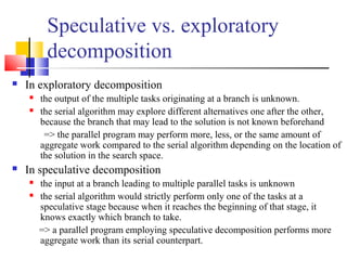
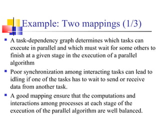
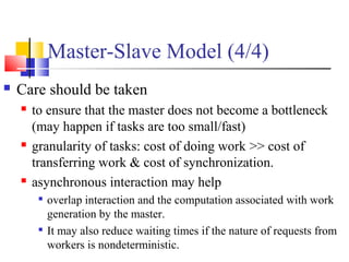
![Task Interaction Graphs: An
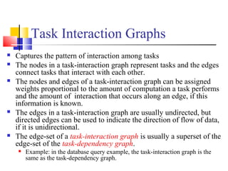
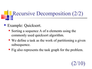
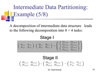
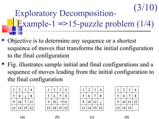
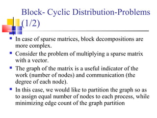
Example (1/3)
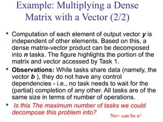
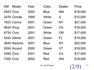
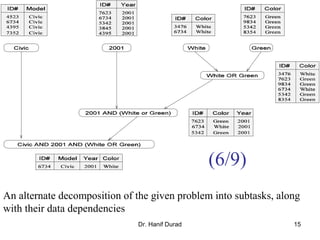
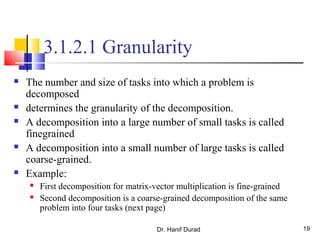
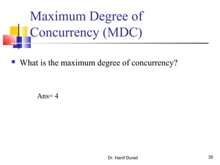
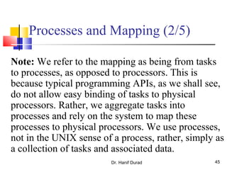
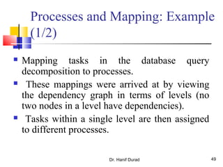
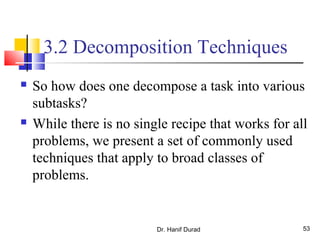
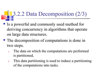
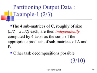
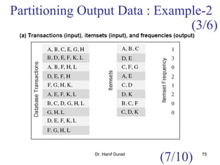
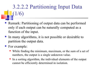
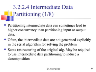
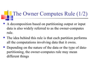
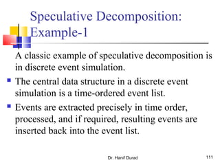
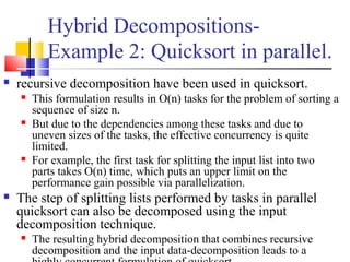
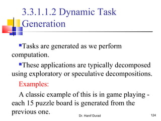
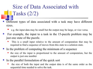
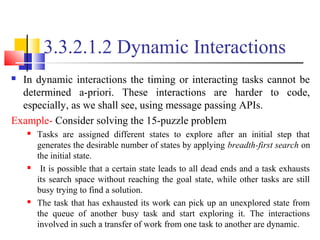
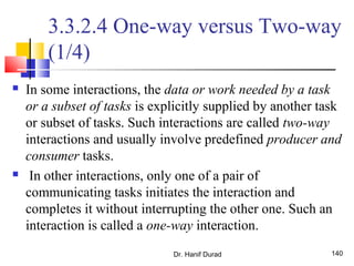
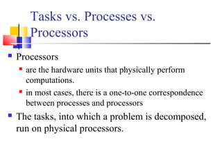
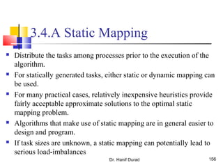
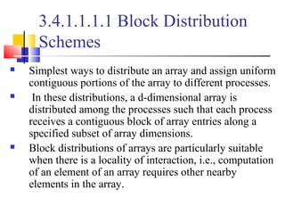
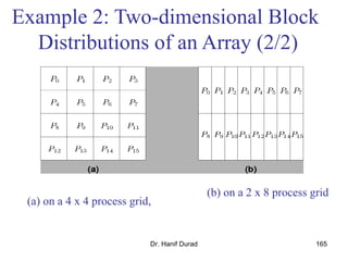
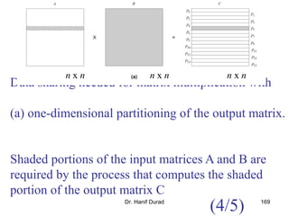
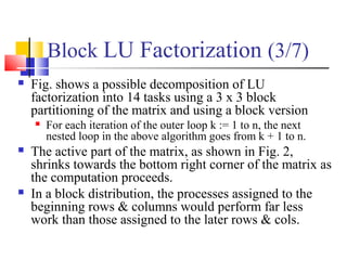
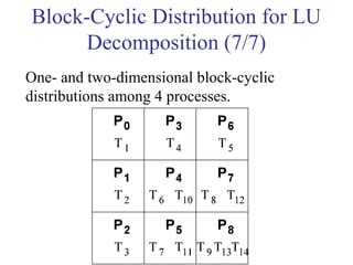
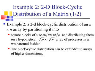
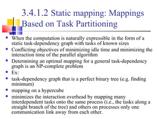
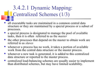
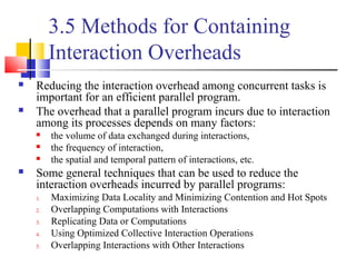
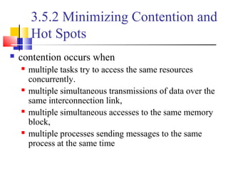
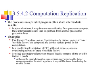
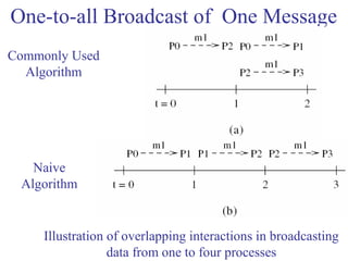
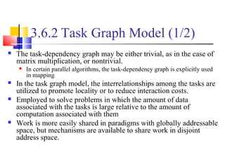
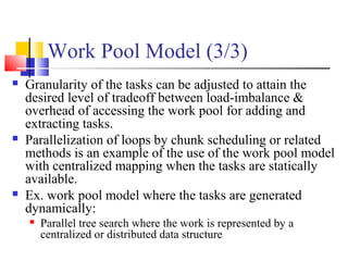
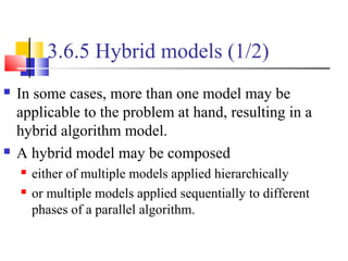
Consider: ? the product y = Ab of a sparse n x n matrix A with a
dense nx1 vector b.
A matrix is considered sparse when a significant no. entries in it
are zero and the locations of the non-zero entries do not conform
to a predefined structure or pattern.
Arithmetic operations involving sparse matrices can often be
optimized significantly by avoiding computations involving the
zeros.
While computing the ith entry of the product vector,
we need to compute the products for only those values
of j for which not equal with 0.
For example, y[0] = A[0, 0].b[0] + A[0, 1].b[1] + A[0, 4].b[4] + A[0,
8].b[8].
y[i]= (A[i,j]b[j])1
n
j∑ =
A[i,j]b[j]
A[i,j]](https://image.slidesharecdn.com/chapter3pc-150609040916-lva1-app6891/85/Chapter-3-pc-40-320.jpg)
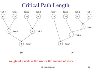
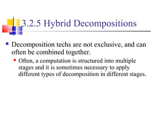
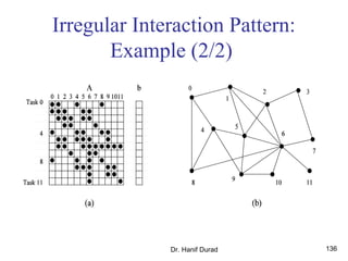
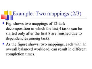
![Task Interaction Graphs: An
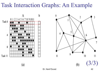
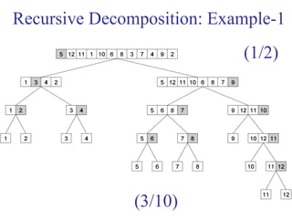
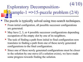
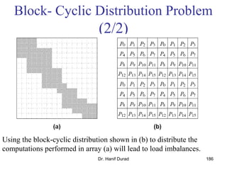
Example (2/3)
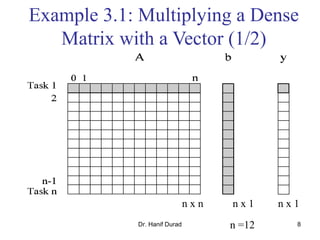
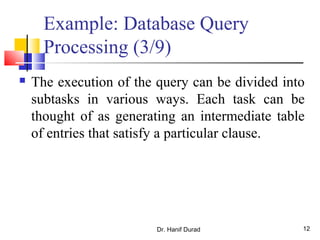
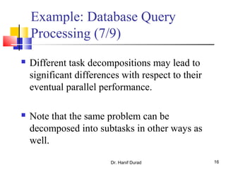
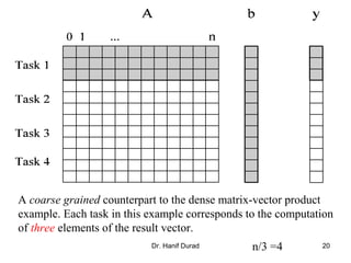
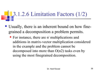
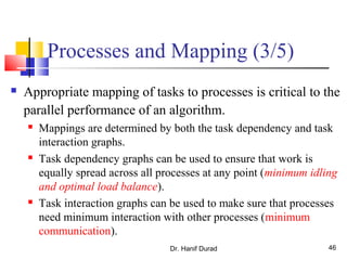
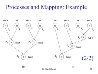
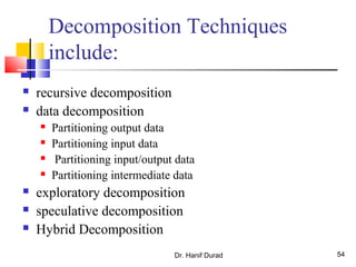
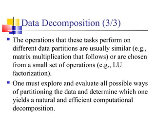
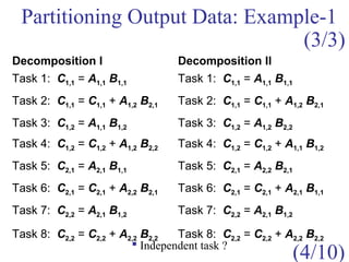
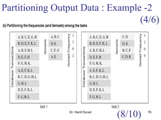
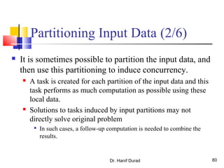
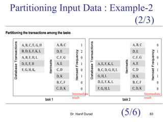
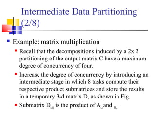
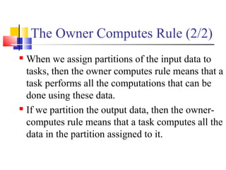
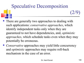
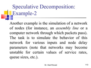
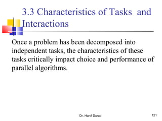
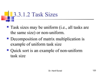
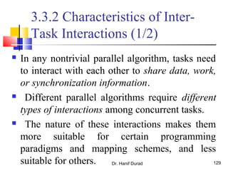
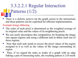
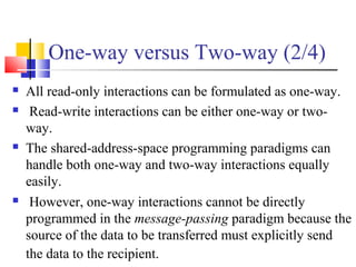
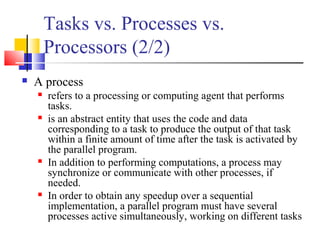
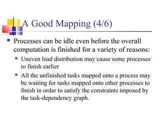
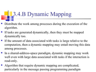
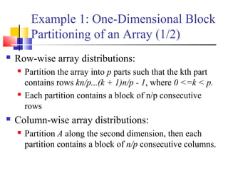
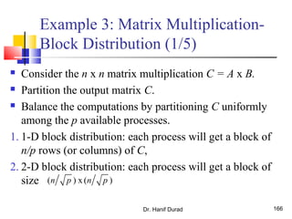
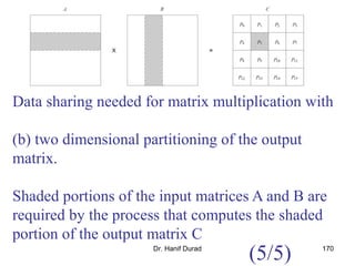
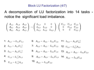
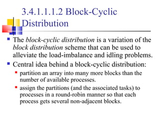
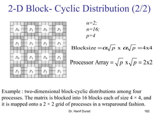
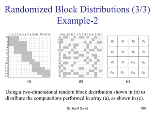
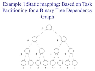
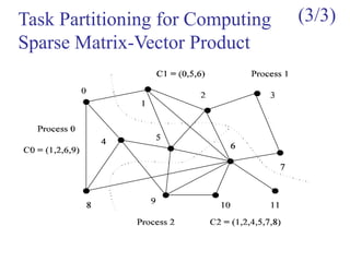
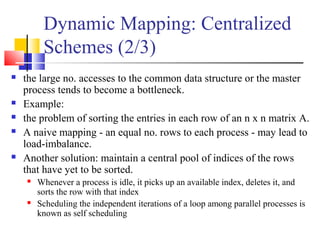
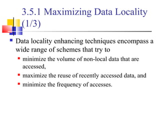
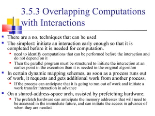
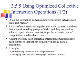
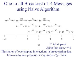
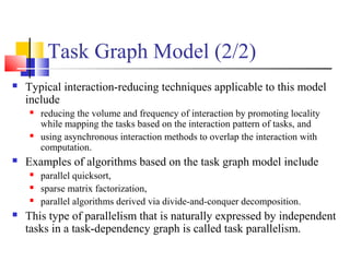
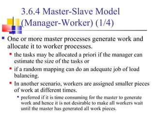
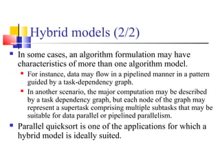
One possible way of decomposing this computation is to partition the
output vector y and have each task compute an entry in it (Fig. (a))
Assigning the computation of the element y[i] of the output vector to Task i,
Task i is the "owner" of row A[i, *] of the matrix and the element b[i] of the
input vector.
The computation of y[i] requires access to many elements of b that are owned
by other tasks
So Task i must get these elements from the appropriate locations.
In the message-passing paradigm, with the ownership of b[i],Task i also inherits the
responsibility of sending b[i] to all the other tasks that need it for their computation.
For example: Task 4 must send b[4] to Tasks 0, 5, 8, and 9 and must get b[0], b[5],
b[8], and b[9] to perform its own computation.](https://image.slidesharecdn.com/chapter3pc-150609040916-lva1-app6891/85/Chapter-3-pc-41-320.jpg)
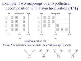
![Dr. Hanif Durad 61
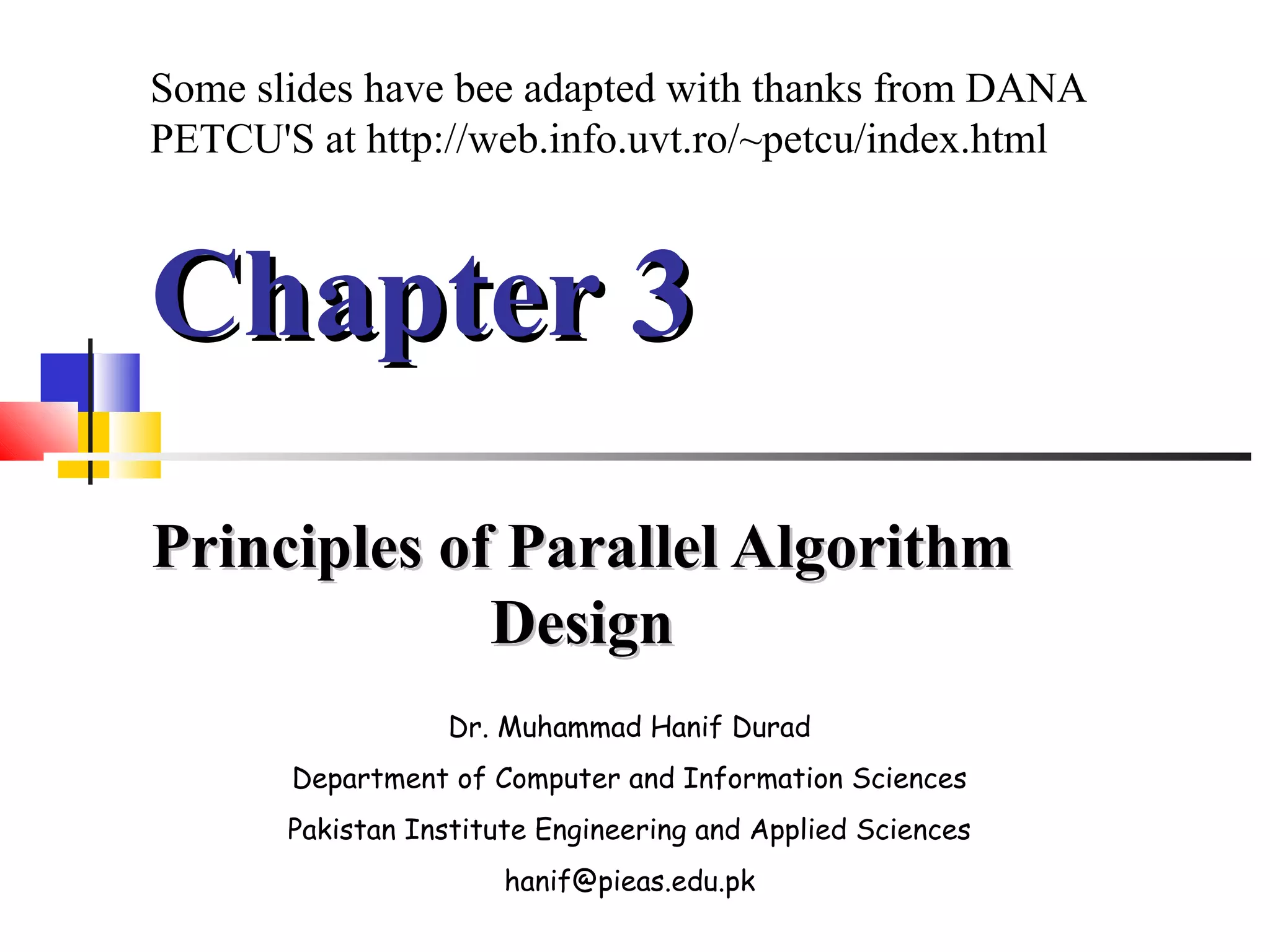
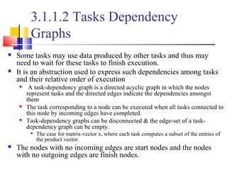
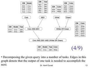
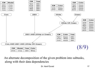
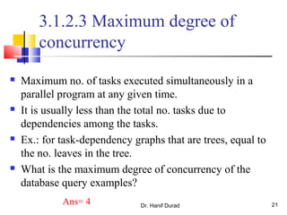
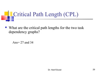
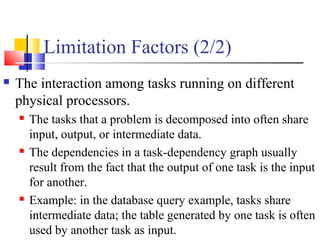
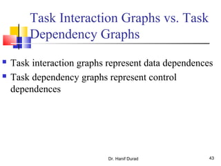
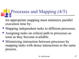
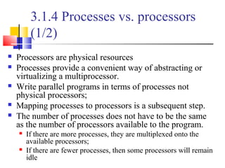
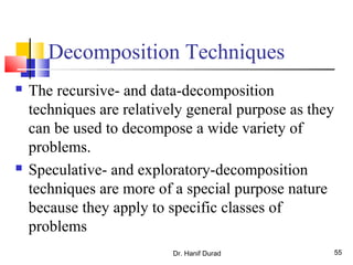
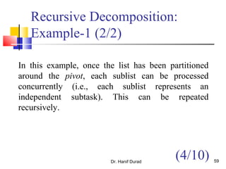
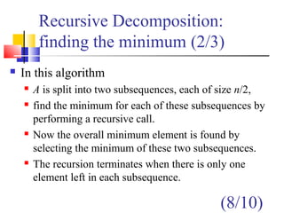
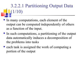
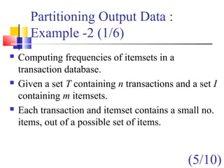
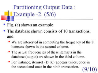
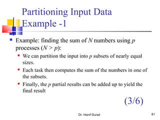
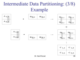
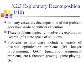
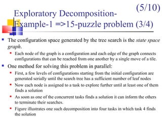
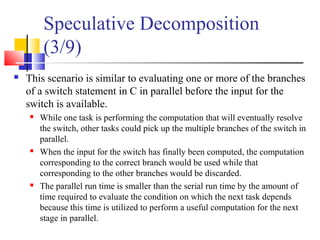
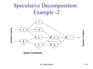
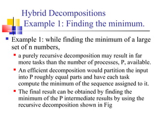
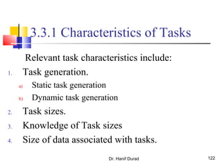
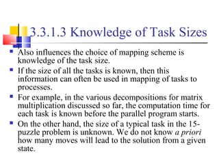
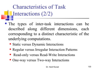
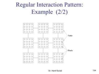
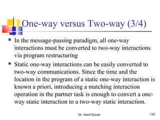
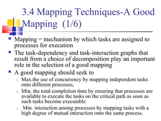
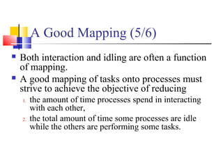
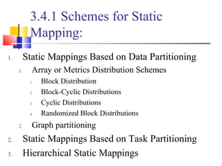
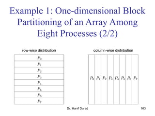
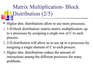
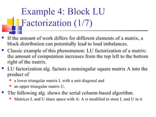
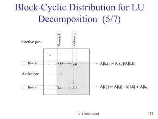
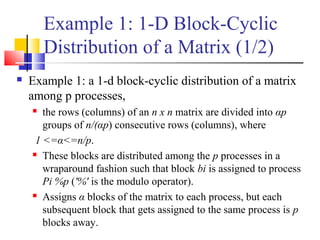
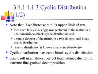
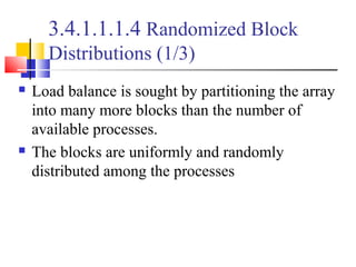
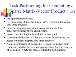
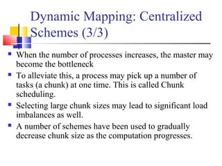
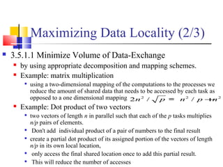
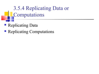
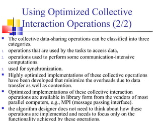
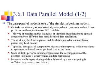
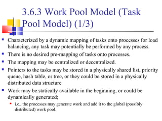
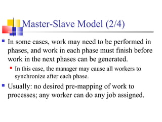
Recursive Decomposition: Example
1. procedure SERIAL_MIN (A,n)
2. begin
3. min = A[0];
4. for i:= 1 to n−1 do
5. if (A[i] <min) min := A[i];
6. endfor;
7. return min;
8. end SERIAL_MIN
(6/10)](https://image.slidesharecdn.com/chapter3pc-150609040916-lva1-app6891/85/Chapter-3-pc-61-320.jpg)
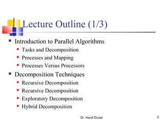
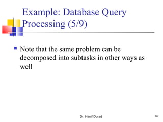
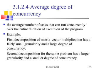
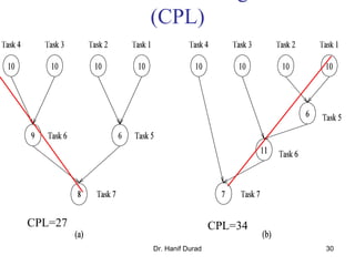
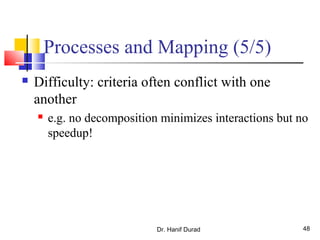
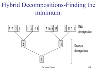
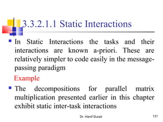
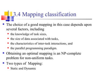
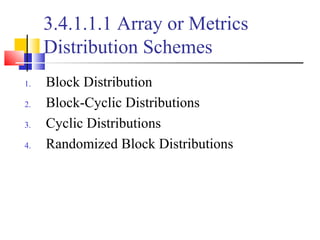
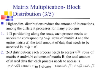
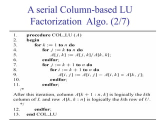
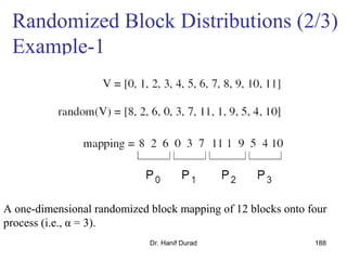
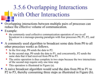
![Recursive Decomposition:
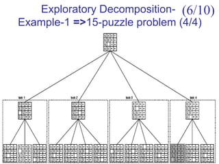
Example
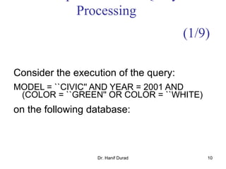
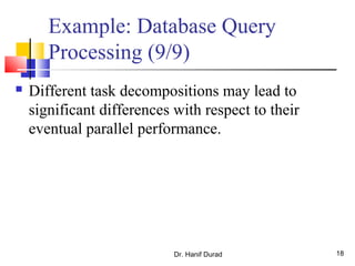
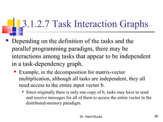
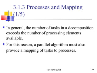
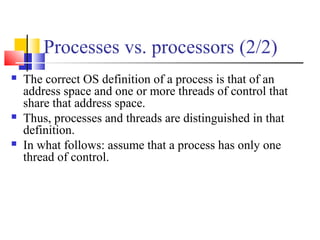
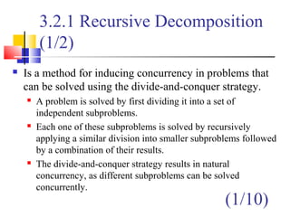
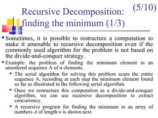
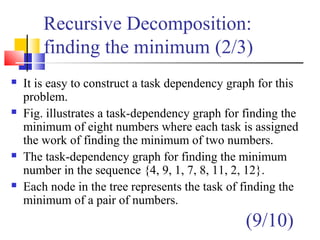
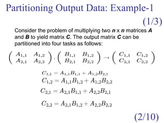
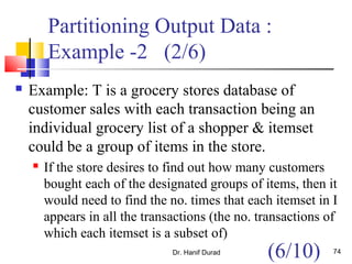
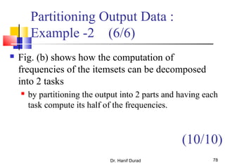
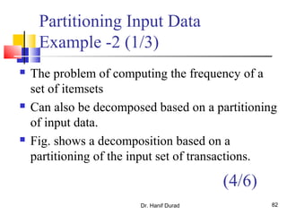
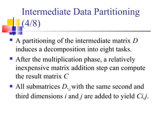
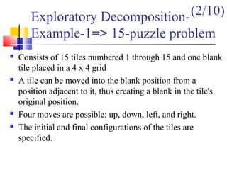
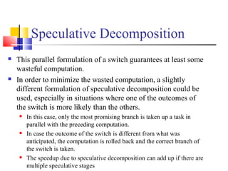
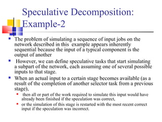
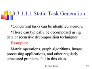
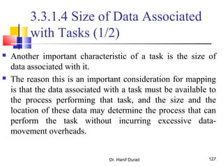
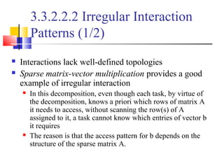
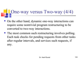
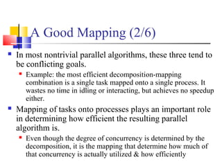
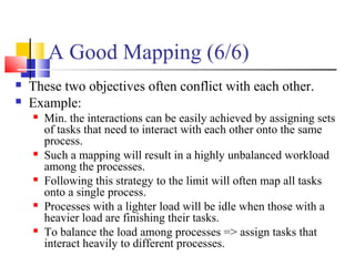
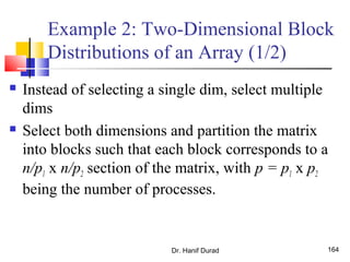
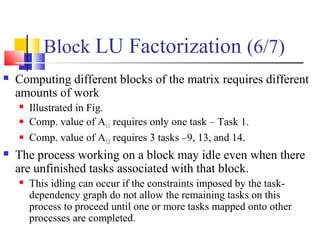
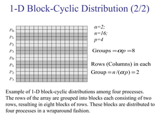
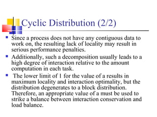
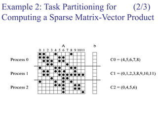
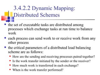
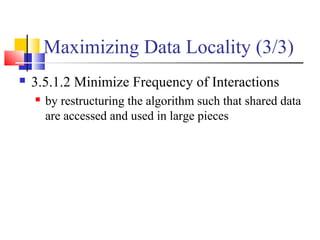
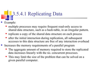
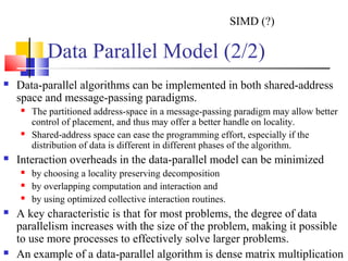
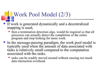
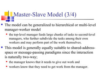
We can rewrite the loop as follows:
1. procedure RECURSIVE_MIN (A, n)
2. begin
3. if ( n = 1 ) then
4. min := A [0] ;
5. else
6. lmin := RECURSIVE_MIN ( A, n/2 );
7. rmin := RECURSIVE_MIN ( &(A[n/2]), n - n/2 );
8. if (lmin < rmin) then
9. min := lmin;
10. else
11. min := rmin;
12. endelse;
13. endelse;
14. return min;
15. end RECURSIVE_MIN
(7/10)](https://image.slidesharecdn.com/chapter3pc-150609040916-lva1-app6891/85/Chapter-3-pc-62-320.jpg)


This document outlines principles of parallel algorithm design. It discusses tasks and decomposition, processes and mapping tasks to processes. Different techniques for decomposing problems are covered, including recursive, exploratory, and hybrid decomposition. Characteristics of tasks such as granularity, concurrency, and interactions are defined. Mapping techniques can help balance load and minimize communication overheads between tasks. Different parallel algorithm design models are also introduced.