Downloaded 17 times


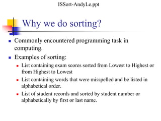


![Insertion sort
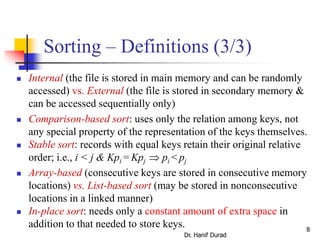
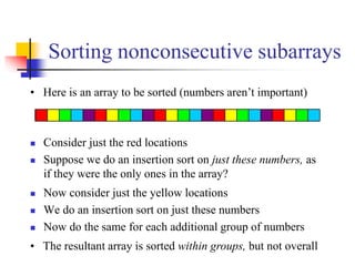
INSERTION-SORT (A, n) ⊳ A[1 . . n]
for j ← 2 to n
do key ← A[ j]
i ← j – 1
while i > 0 and A[i] > key
do A[i+1] ← A[i]
i ← i – 1
A[i+1] = key
“pseudocode”
i j
key
sorted
A:
1 n
Dr. Hanif Durad](https://image.slidesharecdn.com/chapter4ds-190904110928/85/Chapter-4-ds-11-320.jpg)
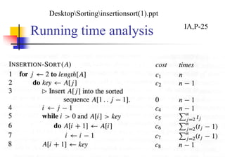
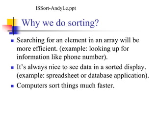
![Some explanation
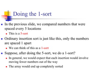
“times” column refers to how many times
each stmt is executed (max)
n = length[A]
tj = # times the while loop test in line 5 is
executed for that value of the index j](https://image.slidesharecdn.com/chapter4ds-190904110928/85/Chapter-4-ds-24-320.jpg)
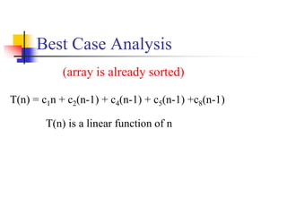
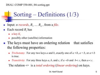
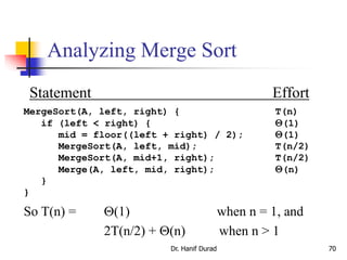
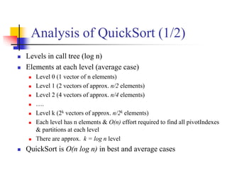
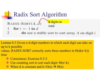
![Worst Case Analysis
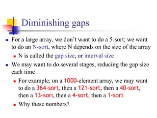
So T(j) = j, for j = 2,3,…,n
Must compare each element A[j] w/ each element
in the entire sorted subarray A[1..j-1]
Thus, T(n) = c1n + c2(n-1) + c4(n-1) + c5(n(n+1)/2 – 1)
+ c6(n(n-1)/2) + c7(n(n-1)/2) + c8(n-1)
T(n) is a quadratic function of n
(array reverse-sorted)](https://image.slidesharecdn.com/chapter4ds-190904110928/85/Chapter-4-ds-26-320.jpg)
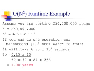


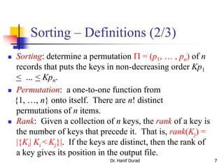
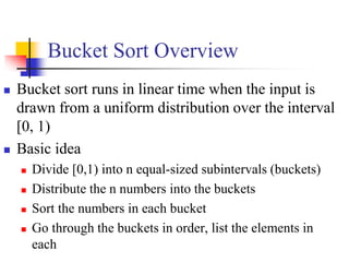
![Shellsort
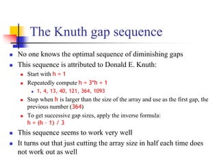
ShellSort(A, n)
1. h 1
2. while h n {
3. h 3h + 1
4. }
5. repeat
6. h h/3
7. for i = h to n do {
8. key A[i]
9. j i
10. while key < A[j - h] {
11. A[j] A[j - h]
12. j j - h
13. if j < h then break
14. }
15. A[j] key
16. }
17. until h 1
Comp 122
When h=1, this is insertion sort.
Otherwise, performs insertion
sort on keys h locations apart.
h values are set in the outermost
repeat loop. Note that they are
decreasing and the final value is 1.
DSAL COMP 550-001, 04-sorting.ppt](https://image.slidesharecdn.com/chapter4ds-190904110928/85/Chapter-4-ds-34-320.jpg)


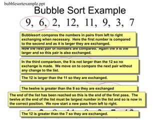
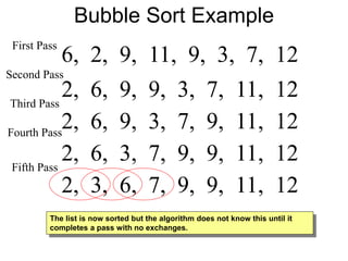
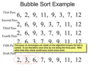
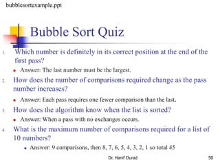
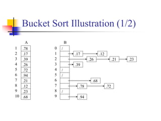
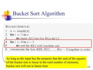
![Bubble Sort Algortithm
1. for i←1 to length[A]
2. for j←length[A] down to i+1
3. if (A[j] < A[j-1])
4. swap(A[j] ,A[j-1]);
Dr. Hanif Durad 47
DS-1, P-453](https://image.slidesharecdn.com/chapter4ds-190904110928/85/Chapter-4-ds-47-320.jpg)

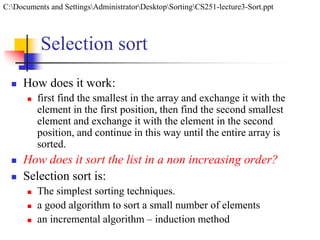
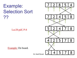
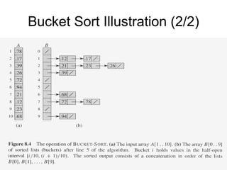
![Selection Sort Algorithm
Input: An array A[1..n] of n elements.
Output: A[1..n] sorted in nondecreasing order.
1. for i 1 to n - 1
2. k i
3. for j i + 1 to n {Find the i th smallest element.}
4. if A[j] < A[k] then k j
5. end for
6. if k i then interchange A[i] and A[k]
7. end for](https://image.slidesharecdn.com/chapter4ds-190904110928/85/Chapter-4-ds-54-320.jpg)


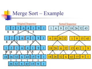
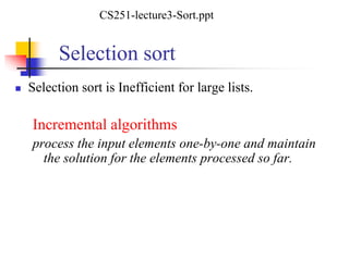
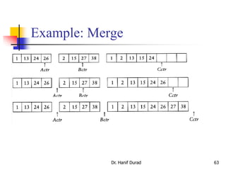
![How to merge two Arrays?
Dr. Hanif Durad 61
Input: two sorted array A and B
Output: an output sorted array C
Three counters: Actr, Bctr, and Cctr
initially set to the beginning of their respective arrays
(1) The smaller of A[Actr] and B[Bctr] is copied to the next entry in C,
and the appropriate counters are advanced
(2) When either input list is exhausted, the remainder of the other list is
copied to C
D:DSALCOMP171 Data Structures and Algorithmmergesort.ppt](https://image.slidesharecdn.com/chapter4ds-190904110928/85/Chapter-4-ds-61-320.jpg)
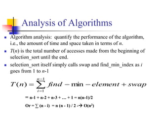
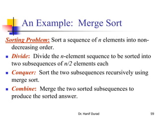
![Merge Sort Algorithm
The procedure MERGE-SORT(A, p, r) sorts the elements in the
sub-array A[ p…r].
The divide step simply computes an index q that partitions A[ p…r]
into two sub-arrays: A[ p…q], containing n/2 elements, and A[ q +
1…r], containing n/2 elements.
To sort the entire sequence A ={A[1], A[2], . . . ,
A[ n]}, we make the initial call MERGE-SORT( A, 1, length[ A]),
where length[ A] = n.
02_Getting Started_2.ppt](https://image.slidesharecdn.com/chapter4ds-190904110928/85/Chapter-4-ds-65-320.jpg)
![L1.66
66
// Copy A[p, q] to L
// Copy A[q+1, r] to R
// Compute # of elements in L
// Compute # of elements in R
// Put a sentinel card at the end of L
// Put a sentinel card at the end of R
// Put the smaller of
L[i] and R[j] to A[K
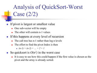
unit03.ppt](https://image.slidesharecdn.com/chapter4ds-190904110928/85/Chapter-4-ds-66-320.jpg)
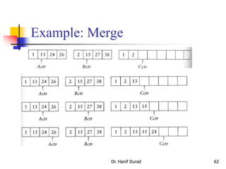
![67
Merge Sort
The key operation of the merge sort algorithm is the
merging of two sorted sequences in the "combine" step. To
perform the merging, we use an auxiliary procedure
MERGE(A, p, q, r), where A is an array and p, q, and r
are indices numbering elements of the array such that p ≤ q
< r.
The procedure assumes that the sub-arrays A[ p…q] and
A[ q + 1…r] are in sorted order. It merges them to form a
single sorted sub-array that replaces the current sub-array
A[ p…r].](https://image.slidesharecdn.com/chapter4ds-190904110928/85/Chapter-4-ds-67-320.jpg)
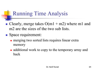
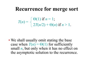
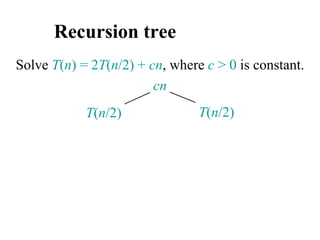
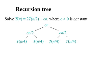
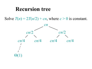
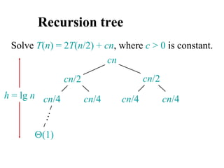
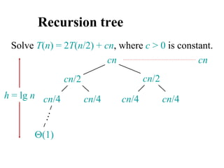
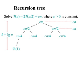
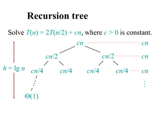
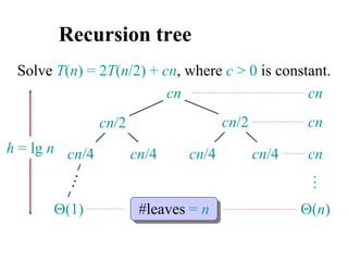
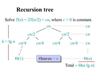
![Analyzing merge sort
MERGE-SORT A[1 . . n]
1. If n = 1, done.
2. Recursively sort A[ 1 . . n/2 ]
and A[ n/2+1 . . n ] .
3. “Merge” the 2 sorted lists
T(n)
(1)
2T(n/2)
(n)
Sloppiness: Should be T( n/2 ) + T( n/2 ) ,
but it turns out not to matter asymptotically.](https://image.slidesharecdn.com/chapter4ds-190904110928/85/Chapter-4-ds-71-320.jpg)

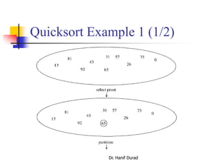
![Introduction
Another divide-and-conquer recursive algorithm, like
mergesort
Quicksort pros [advantage]:
Sorts in place
Sorts O(n lg n) in the average case
Very efficient in practice , it’s quick
Quicksort cons [disadvantage]:
Sorts O(n2) in the worst case
And the worst case doesn’t happen often … sorted
Dr. Hanif Durad 87
D:DSALCOMP171 Data Structures and Algorithmqsort.ppt
C:Documents and SettingsAdministratorDesktopSortingquicksortalgo_Lecture 6 quick_sor.ppt](https://image.slidesharecdn.com/chapter4ds-190904110928/85/Chapter-4-ds-87-320.jpg)
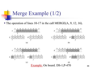
![Quicksort Example 2 (1/7)
150 300 650 550 800 400 350 450
scanUp scanDown
v[0] v[9]v[8]v[7]v[6]v[5]v[4]v[3]v[2]v[1]
pivot
500 900
The quicksort algorithm uses a series of recursive calls to partition a
list into smaller and smaller sublists about a value called the pivot.
Example: Let v be a vector containing 10 integer values:
v = {800, 150, 300, 650, 550, 500, 400, 350, 450,
900}
D:DSALCLRlect6
Dr. Hanif Durad](https://image.slidesharecdn.com/chapter4ds-190904110928/85/Chapter-4-ds-91-320.jpg)
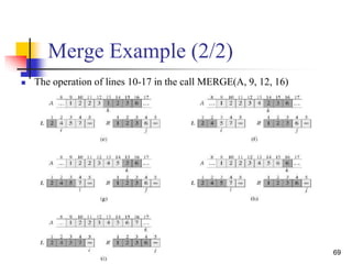
![Quicksort Example 2 (3/7)
Before the exchange
After the exchange and updates to scanUp and scanDown
150 300 650 550 800 400 350 450
scanUp scanDown
v[0] v[9]v[8]v[7]v[6]v[5]v[4]v[3]v[2]v[1]
pivot
500 900
150 300 450 550 800 400 350 650
scanUp scanDown
v[0] v[9]v[8]v[7]v[6]v[5]v[4]v[3]v[2]v[1]
pivot
500 900
Dr. Hanif Durad](https://image.slidesharecdn.com/chapter4ds-190904110928/85/Chapter-4-ds-92-320.jpg)
![Quicksort Example 2 (3/7)
Before the exchange
After the exchange and updates to scanUp and scanDown
150 300 450 550 800 400 350 650
scanUp scanDown
v[0] v[9]v[8]v[7]v[6]v[5]v[4]v[3]v[2]v[1]
pivot
500 900
150 300 450 350 800 400 550 650
scanUp scanDown
v[0] v[9]v[8]v[7]v[6]v[5]v[4]v[3]v[2]v[1]
pivot
500 900
Dr. Hanif Durad](https://image.slidesharecdn.com/chapter4ds-190904110928/85/Chapter-4-ds-93-320.jpg)
![Quicksort Example 2 (4/7)
Before the exchange
After the exchange and updates to scanUp and scanDown
150 300 450 350 800 400 550 650
scanUp scanDown
v[0] v[9]v[8]v[7]v[6]v[5]v[4]v[3]v[2]v[1]
pivot
500 900
150 300 450 350 400 800 550 650
scanUpscanDown
v[0] v[9]v[8]v[7]v[6]v[5]v[4]v[3]v[2]v[1]
pivot
500 900
Dr. Hanif Durad](https://image.slidesharecdn.com/chapter4ds-190904110928/85/Chapter-4-ds-94-320.jpg)
![Quicksort Example 2 (4/7)
400 150 300 450 350 500 800 550 650
v[0] v[9]v[8]v[7]v[6]v[5]v[4]v[3]v[2]v[1]
900
Pivot in its final position
400 150 300 450 350 500 800 550 650
v[0] v[9]v[8]v[7]v[6]v[5]v[4]v[3]v[2]v[1]
v[0] - v[4] v[6] - v[9]
900
Dr. Hanif Durad](https://image.slidesharecdn.com/chapter4ds-190904110928/85/Chapter-4-ds-95-320.jpg)
![Quicksort Example 2 (5/7)
pivot
300 150 400 450 350
scanUp
v[0] v[4]v[3]v[2]v[1]
Initial Values
scanDown
pivot
300 150 400 450 350
v[0] v[4]v[3]v[2]v[1]
scanUp
After Scans Stop
scanDown
150 300 400 450 350
v[0] v[4]v[3]v[2]v[1]
Dr. Hanif Durad](https://image.slidesharecdn.com/chapter4ds-190904110928/85/Chapter-4-ds-96-320.jpg)
![pivot
650 550 800 900
scanUp
v[6] v[9]v[8]v[7]
Initial Values
scanDown
pivot
650 550 800 900
v[6] v[9]v[8]v[7]
scanUp
After Stops
scanDown
550 650 800 900
v[6] v[9]v[8]v[7]
Quicksort Example 2 (6/7)
Dr. Hanif Durad](https://image.slidesharecdn.com/chapter4ds-190904110928/85/Chapter-4-ds-97-320.jpg)
![Quicksort Example 2 (7/7)
v[0] v[4]v[3]v[2]v[1] v[6] v[9]v[8]v[7]v[5]
150 900800650550500350450400300
400 450 350
v[4]v[3]v[2]
Before Partitioning
350 400 450
v[4]v[3]v[2]
After Partitioning
150 300 350 400 450 500
v[0] v[4]v[3]v[2]v[1]
550 650 800 900
v[6] v[9]v[8]v[7]v[5]
Dr. Hanif Durad](https://image.slidesharecdn.com/chapter4ds-190904110928/85/Chapter-4-ds-98-320.jpg)
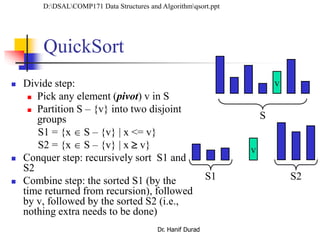
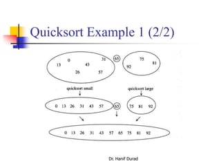
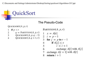
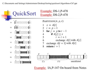
![QuickSort
Like in MERGESORT, we use Divide-and-Conquer:
1. Divide: partition A[p..r] into two subarrays A[p..q-1] and
A[q+1..r] such that each element of A[p..q-1] is ≤ A[q], and each
element of A[q+1..r] is ≥ A[q]. Compute q as part of this
partitioning.
2. Conquer: sort the subarrays A[p..q-1] and A[q+1..r] by recursive
calls to QUICKSORT.
3. Combine: the partitioning and recursive sorting leave us with a
sorted A[p..r] – no work needed here.
An obvious difference is that we do most of the work in the divide
stage, with no work at the combine one.
C:Documents and SettingsAdministratorDesktopSortingquicksortAlgorithms-Ch7.ppt](https://image.slidesharecdn.com/chapter4ds-190904110928/85/Chapter-4-ds-99-320.jpg)
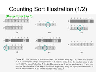
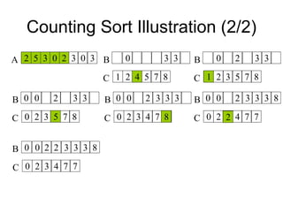
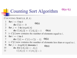
![Counting Sort Overview
Assumption: n input elements are integers in the range of 0
to k (integer).
(n+k) When k=O(n), counting sort: (n)
Basic Idea
For each input element x, determine the number of elements less
than or equal to x
For each integer i (0 i k), count how many elements whose
values are i
Then we know how many elements are less than or equal to i
Algorithm storage
A[1..n]: input elements
B[1..n]: sorted elements
C[0..k]: hold the number of elements less than or equal to i](https://image.slidesharecdn.com/chapter4ds-190904110928/85/Chapter-4-ds-105-320.jpg)
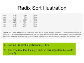
![Counting Sort Is Stable
A sorting algorithm is stable if
Numbers with the same value appear in the output array
in the same order as they do in the input array
Ties between two numbers are broken by the rule that
which ever number appears first in the input array
appears first in the output array
Line 9 of counting sort: for jlength[A] down to 1
is essential for counting sort to be stable
What if for j 1 to length[A]](https://image.slidesharecdn.com/chapter4ds-190904110928/85/Chapter-4-ds-109-320.jpg)


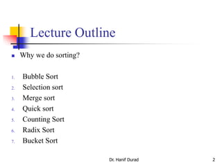
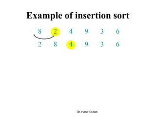
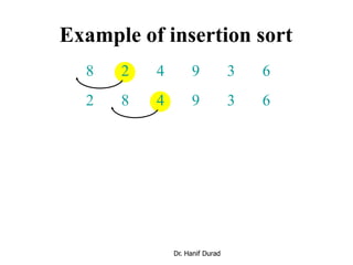
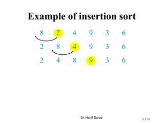
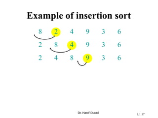
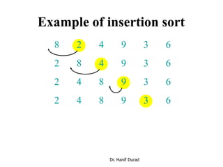
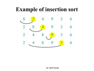
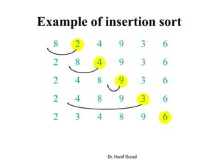
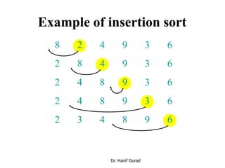
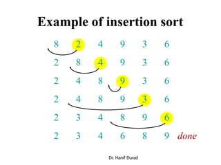
This document provides an overview of sorting algorithms including bubble sort, insertion sort, shellsort, and others. It discusses why sorting is important, provides pseudocode for common sorting algorithms, and gives examples of how each algorithm works on sample data. The runtime of sorting algorithms like insertion sort and shellsort are analyzed, with insertion sort having quadratic runtime in the worst case and shellsort having unknown but likely better than quadratic runtime.