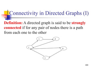
Downloaded 14 times


![Adjacency Lists
Consists of an array Adj of |V| lists.
One list per vertex.
For u V, Adj[u] consists of all vertices adjacent to u.
a
dc
b a
b
c
d
b
c
d
d c
a
dc
b a
b
c
d
b
a
d
d c
c
a b
a c
If weighted, store weights also in
adjacency lists.](https://image.slidesharecdn.com/chapter23aoa-190904110932/85/Chapter-23-aoa-7-320.jpg)


![Adjacency Matrix
V| |V| matrix A.
Number vertices from 1 to |V| in some arbitrary manner.
A is then given by:
a
dc
b
3 4
1 2 3 4
1 0 1 1 1
2 0 0 1 0
3 0 0 0 1
4 0 0 0 0
a
dc
b
1 2
3 4
1 2 3 4
1 0 1 1 1
2 1 0 1 0
3 1 1 0 1
4 1 0 1 0
otherwise0
),(if1
],[
Eji
ajiA ij
A = AT for undirected graphs.](https://image.slidesharecdn.com/chapter23aoa-190904110932/85/Chapter-23-aoa-10-320.jpg)


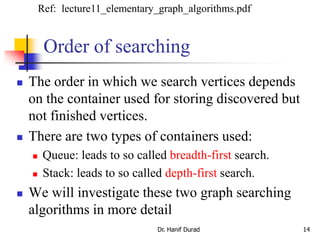

![Breadth-First Search (BFS)
Input: Graph G = (V, E), either directed or undirected,
and source vertex s V.
Output:
d[v] = distance (smallest # of edges, or shortest path) from s
to v, for all v V. d[v] = if v is not reachable from s.
[v] = u such that (u, v) is last edge on “shortest path” from s
to v.
u is v’s predecessor.
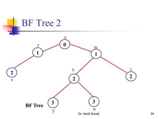
Builds breadth-first tree with root s that contains all reachable
vertices.
16
19-graph1.ppt
Shortest Path- path containing smallest no. of edges](https://image.slidesharecdn.com/chapter23aoa-190904110932/85/Chapter-23-aoa-16-320.jpg)


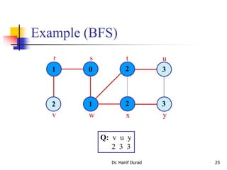
![19
BFS(G,s)
1. for each vertex u in V[G] – {s}
2 do color[u] white
3 d[u]
4 [u] nil
5 color[s] gray
6 d[s] 0
7 [s] nil
8 Q
9 enqueue(Q,s)
10 while Q
11 do u dequeue(Q)
12 for each v in Adj[u]
13 do if color[v] = white
14 then color[v] gray
15 d[v] d[u] + 1
16 [v] u
17 enqueue(Q,v)
18 color[u] black
white: undiscovered
gray: discovered
black: finished
Q: a queue of discovered
vertices
color[v]: color of v
d[v]: distance from s to v
[u]: predecessor of v
Example: animation.
Initialization
Set up s and initialize Q
Explore all the vertices
adjacent to u and update
d, and Q](https://image.slidesharecdn.com/chapter23aoa-190904110932/85/Chapter-23-aoa-19-320.jpg)


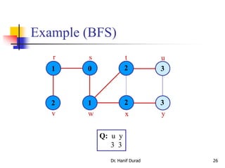


![Data Structure for DFS
Adjacency list
color[u] for each vertex
WHITE if u has not been discovered
GRAY if u is discovered but not finished
BLACK if u is finished
Timestamps: 1 d[u] < f[u] 2|V|
d[u] records when u is first discovered (and grayed)
f[u] records when the search finishes examining u’s
adjacency list (and blacken u)
[u] for predecessor of u
unit14.ppt](https://image.slidesharecdn.com/chapter23aoa-190904110932/85/Chapter-23-aoa-41-320.jpg)
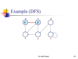
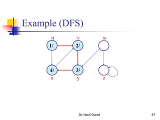
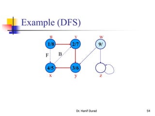
![Depth-first Search (DFS)
Input: G = (V, E), directed or undirected. No source
vertex given!
Output:
2 timestamps on each vertex. Integers between 1 and
2|V|.
d[v] = discovery time (v turns from white to gray)
f [v] = finishing time (v turns from gray to black)
[v] : predecessor of v = u, such that v was discovered
during the scan of u’s adjacency list.
Uses the same coloring scheme for vertices as BFS.
19-graph1.ppt](https://image.slidesharecdn.com/chapter23aoa-190904110932/85/Chapter-23-aoa-42-320.jpg)
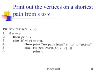
![Pseudo-code
DFS(G)
1. for each vertex u V[G]
2. do color[u] white
3. [u] NIL
4. time 0
5. for each vertex u V[G]
6. do if color[u] = white
7. then DFS-Visit(u)
Uses a global timestamp time.
DFS-Visit(u)
1. color[u] GRAY White vertex u
has been discovered
2. time time + 1
3. d[u] time
4. for each v Adj[u]
5. do if color[v] = WHITE
6. then [v] u
7. DFS-Visit(v)
8. color[u] BLACK Blacken u;
it is finished.
9. f[u] time time + 1
Example: animation.
43
Init all
vertices
Visit all
children
recursively
Dr. Hanif Durad](https://image.slidesharecdn.com/chapter23aoa-190904110932/85/Chapter-23-aoa-43-320.jpg)


![Analysis of DFS
Loops on lines 1-2 & 5-7 take (V) time,
excluding time to execute DFS-Visit.
DFS-Visit is called once for each white vertex vV
when it’s painted gray the first time. Lines 3-6 of
DFS-Visit is executed |Adj[v]| times. The total
cost of executing DFS-Visit is vV|Adj[v]| = (E)
Total running time of DFS is (V+E).
Dr. Hanif Durad 60](https://image.slidesharecdn.com/chapter23aoa-190904110932/85/Chapter-23-aoa-60-320.jpg)

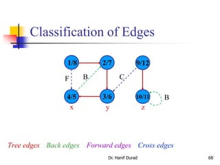
![Depth-First Trees
Predecessor subgraph defined slightly different from
that of BFS.
The predecessor subgraph of DFS is G = (V, E) where
E ={([v],v) : v V and [v] NIL}.
How does it differ from that of BFS?
The predecessor subgraph G forms a depth-first forest
composed of several depth-first trees. The edges in E are
called tree edges.
Dr. Hanif Durad 62
Definition:
Forest: An acyclic graph G that may be disconnected.](https://image.slidesharecdn.com/chapter23aoa-190904110932/85/Chapter-23-aoa-62-320.jpg)

![Theorem 22.7
For all u, v, exactly one of the following holds:
1. d[u] < f [u] < d[v] < f [v] or d[v] < f [v] < d[u] < f [u] and neither
u nor v is a descendant of the other.
2. d[u] < d[v] < f [v] < f [u] and v is a descendant of u.
3. d[v] < d[u] < f [u] < f [v] and u is a descendant of v.
So d[u] < d[v] < f [u] < f [v] cannot happen.
Like parentheses:
OK: ( ) [ ] ( [ ] ) [ ( ) ]
Not OK: ( [ ) ] [ ( ] )
Corollary
v is a proper descendant of u if and only if d[u] < d[v] < f [v] < f [u].
Parenthesis Theorem
19-graph1.ppt](https://image.slidesharecdn.com/chapter23aoa-190904110932/85/Chapter-23-aoa-64-320.jpg)


![Topological Sort
Dr. Hanif Durad 75
Topological-Sort (G)
1. call DFS(G) to compute finishing times f [v] for all v V
2. as each vertex is finished, insert it onto the front of a linked
list
3. return the linked list of vertices
Time: (V + E).
20-graph2.ppt](https://image.slidesharecdn.com/chapter23aoa-190904110932/85/Chapter-23-aoa-75-320.jpg)

![Characterizing a DAG (2/2)
Proof (Contd.): : Show that a cycle implies a back edge.
c : cycle in G, v : first vertex discovered in c, (u, v) : preceding
edge in c.
At time d[v], vertices of c form a white path v u. Why?
By white-path theorem, u is a descendent of v in depth-first forest.
Therefore, (u, v) is a back edge.
77
Lemma 22.11
A directed graph G is acyclic iff a DFS of G yields no back edges.
v u
T T T
B
20-graph2.ppt](https://image.slidesharecdn.com/chapter23aoa-190904110932/85/Chapter-23-aoa-77-320.jpg)

![Theorem 22.12
• TOPOLOGICAL-SORT(G) produces a
topological sort of a directed acyclic graph G
– Suppose that DFS is run on a given DAG G to determine
finishing times for its vertices. It suffices to show that for
any pair of distinct vertices u, v, if there is an edge in G
from u to v, then f[v] < f[u].
• The linear ordering is corresponding to finishing time ordering
– Consider any edge (u, v) explored by DFS(G). When this
edge is explored, v cannot be gray (otherwise, (u, v) will be
a back edge). Therefore v must be either white or black
• If v is white, v becomes a descendant of u, f[v] <f[u] (ex. pants &
shoes)
• If v is black, it has already been finished, so that f[v] has already
been set f[v] < f[u] (ex. belt & jacket)
Dr. Hanif Durad 79
Self Study](https://image.slidesharecdn.com/chapter23aoa-190904110932/85/Chapter-23-aoa-79-320.jpg)


![Algorithm to determine SCCs
Dr. Hanif Durad 85
SCC(G)
1. call DFS(G) to compute finishing times f [u] for all u
2. compute GT
3. call DFS(GT), but in the main loop, consider vertices in order of
decreasing f [u] (as computed in first DFS)
4. output the vertices in each tree of the depth-first forest formed in
second DFS as a separate SCC
Time: (V + E).
20-graph2.ppt](https://image.slidesharecdn.com/chapter23aoa-190904110932/85/Chapter-23-aoa-85-320.jpg)
![Example (1/5)
Dr. Hanif Durad 86
(Courtesy of Prof. Jim Anderson)
13/14
12/15 3/4 2/7
11/16 1/10
a b c
e f g
5/6
8/9
h
d
G
Sort nodes on their finishing time:
b,e,a,c,d,g,f,h
1. call DFS(G) to compute finishing times f [u] for all u
20-graph2.ppt
text taken from: lecture11_elementary_graph_algorithms.pdf](https://image.slidesharecdn.com/chapter23aoa-190904110932/85/Chapter-23-aoa-86-320.jpg)

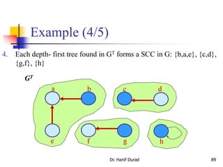
![Example (3/5)
Dr. Hanif Durad 88
(Courtesy of Prof. Jim Anderson)
Deep- first- trees found: {b,a,e}, {c,d}, {g,f}, {h}
3. call DFS(GT), but in the main loop, consider vertices in order of
decreasing f [u] (as computed in line 1 b,e,a,c,d,g,f,h)
a b c
e f g h
d
GT](https://image.slidesharecdn.com/chapter23aoa-190904110932/85/Chapter-23-aoa-88-320.jpg)
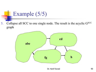
![Analysis of SCC algorithm
1. Call DFS(G) to compute finishing times f[u] for each
vertex u in G Θ(V + E)
2. Compute transpose graph GT Θ(V + E)
3. Call DFS(GT), but in he main loop, consider the
vertices in decreasing f[u] (as computed in line 1)
Θ(V + E)
4. Collapse each depth-first tree found in GT to a SCC
Θ(V + E)
Overall total time: Θ(V + E)
Dr. Hanif Durad 91](https://image.slidesharecdn.com/chapter23aoa-190904110932/85/Chapter-23-aoa-91-320.jpg)


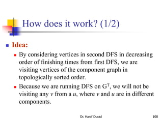
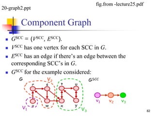
![How does it work? (2/2)
Notation:
d[u] and f [u] always refer to first DFS.
Extend notation for d and f to sets of vertices U V:
d(U) = minuU{d[u]} (earliest discovery time)
f (U) = maxuU{ f [u]} (latest finishing time)
Dr. Hanif Durad 109](https://image.slidesharecdn.com/chapter23aoa-190904110932/85/Chapter-23-aoa-109-320.jpg)
![110
SCCs and DFS finishing times
Proof:
Case 1: d(C) < d(C)
» Let x be the first vertex discovered in
C.
» At time d[x], all vertices in C and C
are white. Thus, there exist paths of
white vertices from x to all vertices in
C and C.
» By the white-path theorem, all
vertices in C and C are descendants
of x in depth-first tree.
» By the parenthesis theorem, f [x] = f
(C) > f(C).
Lemma 22.14
Let C and C be distinct SCC’s in G = (V, E). Suppose there is an
edge (u, v) E such that u C and v C. Then f (C) > f (C).
C C
u v
x](https://image.slidesharecdn.com/chapter23aoa-190904110932/85/Chapter-23-aoa-110-320.jpg)
![111
SCCs and DFS finishing times
Proof:
Case 2: d(C) > d(C)
» Let y be the first vertex discovered in C.
» At time d[y], all vertices in C are white
and there is a white path from y to each
vertex in C all vertices in C become
descendants of y. Again, f [y] = f (C).
» At time d[y], all vertices in C are also
white.
» By earlier lemma, since there is an edge
(u, v), we cannot have a path from C to
C.
» So no vertex in C is reachable from y.
» Therefore, at time f [y], all vertices in C
are still white.
» Therefore, for all w C, f [w] > f [y],
which implies that f (C) > f (C).
Lemma 22.14
Let C and C be distinct SCC’s in G = (V, E). Suppose there is an
edge (u, v) E such that u C and v C. Then f (C) > f (C).
C C
u v
yx](https://image.slidesharecdn.com/chapter23aoa-190904110932/85/Chapter-23-aoa-111-320.jpg)


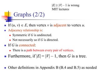
This document provides an outline and overview of a lecture on elementary graph algorithms. It begins with contact information for the lecturer, Dr. Muhammad Hanif Durad. It then outlines topics to be covered, including definition and representation of graphs, breadth-first search, depth-first search, topological sort, and strongly connected components. The document discusses the importance of graphs and examples of problems that can be modeled with graphs. It provides definitions and descriptions of basic graph terminology like vertices, edges, types of graphs. It also covers representations of graphs using adjacency lists and adjacency matrices. The document dives deeper into breadth-first search and depth-first search algorithms, providing pseudocode and examples. It discusses applications and analysis of the algorithms.