Downloaded 13 times

![9.2 Binary Search Tree Property
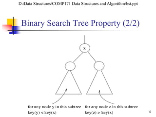
(1/2)
Stored keys must satisfy
the binary search tree
property.
y in left subtree of x,
then key[y] key[x].
y in right subtree of x,
then key[y] key[x].
56
26 200
18 28 190 213
12 24 27](https://image.slidesharecdn.com/chapter9ds-190904110931/85/Chapter-9-ds-5-320.jpg)
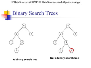
![BST – Representation
Represented by a linked data structure of
nodes.
root(T) points to the root of tree T.
Each node contains fields:
key
left – pointer to left child: root of left subtree.
right – pointer to right child : root of right subtree.
p – pointer to parent. p[root[T]] = NIL (optional).
Rightleft
key
Parent
D:DSALCOMP 550-00115-btrees.ppt](https://image.slidesharecdn.com/chapter9ds-190904110931/85/Chapter-9-ds-8-320.jpg)
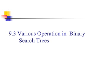
![Inorder Traversal (1/2)
Inorder-Tree-Walk (x)
1. if x NIL
2. then Inorder-Tree-Walk(left[p])
3. print key[x]
4. Inorder-Tree-Walk(right[p])
The binary-search-tree property allows the keys of a binary search
tree to be printed, in (monotonically increasing) order, recursively.
D:DSALCOMP 550-00115-btrees.ppt](https://image.slidesharecdn.com/chapter9ds-190904110931/85/Chapter-9-ds-10-320.jpg)
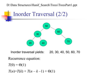
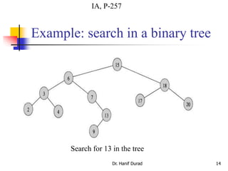
![Tree Search
Tree-Search(x, k)
1. if x = NIL or k = key[x]
2. then return x
3. if k < key[x]
4. then return Tree-Search(left[x], k)
5. else return Tree-Search(right[x], k)
Running time: O(h)
56
26 200
18 28 190 213
12 24 27
IA, P-256](https://image.slidesharecdn.com/chapter9ds-190904110931/85/Chapter-9-ds-13-320.jpg)
![Iterative Tree Search
Iterative-Tree-Search(x, k)
1. while x NIL and k key[x]
2. do if k < key[x]
3. then x left[x]
4. else x right[x]
5. return x
The iterative tree search is more efficient on most computers.
The recursive tree search is more straightforward.
56
26 200
18 28 190 213
12 24 27](https://image.slidesharecdn.com/chapter9ds-190904110931/85/Chapter-9-ds-15-320.jpg)
![Finding Min & Max
Tree-Minimum(x) Tree-Maximum(x)
1. while left[x] NIL 1. while right[x] NIL
2. do x left[x] 2. do x right[x]
3. return x 3. return x
Q: How long do they take?
The binary-search-tree property guarantees that:
The minimum is located at the left-most node.
The maximum is located at the right-most node.](https://image.slidesharecdn.com/chapter9ds-190904110931/85/Chapter-9-ds-16-320.jpg)
![Predecessor and Successor
Successor of node x is the node y such that key[y] is
the smallest key greater than key[x].
The successor of the largest key is NIL.
Search consists of two cases.
If node x has a non-empty right subtree, then x’s successor is
the minimum in the right subtree of x.
If node x has an empty right subtree, then:
As long as we move to the left up the tree (move up through right
children), we are visiting smaller keys.
x’s successor y is the node that x is the predecessor of (x is the
maximum in y’s left subtree).
In other words, x’s successor y, is the lowest ancestor of x whose left
child is also an ancestor of x.](https://image.slidesharecdn.com/chapter9ds-190904110931/85/Chapter-9-ds-17-320.jpg)
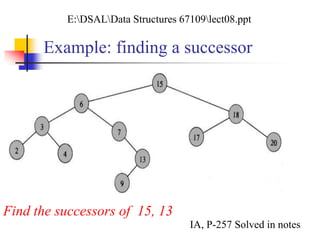
![Pseudo-code for Successor
Code for predecessor is symmetric.
Running time: O(h)
56
26 200
18 28 190 213
12 24 27
Tree-Successor(x)
if right[x] NIL
2. then return Tree-Minimum(right[x])
3. y p[x]
4. while y NIL and x = right[y]
5. do x y
6. y p[y]
7. return y](https://image.slidesharecdn.com/chapter9ds-190904110931/85/Chapter-9-ds-18-320.jpg)
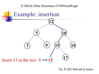
![BST Insertion – Pseudocode
Tree-Insert(T, z)
1. y NIL
2. x root[T]
3. while x NIL
4. do y x
5. if key[z] < key[x]
6. then x left[x]
7. else x right[x]
8. p[z] y
9. if y = NIL
10. then root[t] z
11. else if key[z] < key[y]
12. then left[y] z
13. else right[y] z
Change the dynamic set
represented by a BST.
Ensure the binary-search-
tree property holds after
change.
Insertion is easier than
deletion.
56
26 200
18 28 190 213
12 24 27](https://image.slidesharecdn.com/chapter9ds-190904110931/85/Chapter-9-ds-20-320.jpg)
![Analysis of Insertion
Initialization: O(1)
While loop in lines 3-7
searches for place to
insert z, maintaining
parent y.
This takes O(h) time.
Lines 8-13 insert the
value: O(1)
TOTAL: O(h) time to
insert a node.
Tree-Insert(T, z)
1. y NIL
2. x root[T]
3. while x NIL
4. do y x
5. if key[z] < key[x]
6. then x left[x]
7. else x right[x]
8. p[z] y
9. if y = NIL
10. then root[t] z
11. else if key[z] < key[y]
12. then left[y] z
13. else right[y] z](https://image.slidesharecdn.com/chapter9ds-190904110931/85/Chapter-9-ds-21-320.jpg)
![Exercise: Sorting Using BSTs
Sort (A)
for i 1 to n
do tree-insert(A[i])
inorder-tree-walk(root)
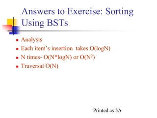
What are the worst case and best case running times?
In practice, how would this compare to other sorting
algorithms?](https://image.slidesharecdn.com/chapter9ds-190904110931/85/Chapter-9-ds-23-320.jpg)
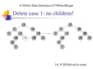
![Tree-Delete (T, x)
if x has no children case 0
then remove x
if x has one child case 1
then make p[x] point to child
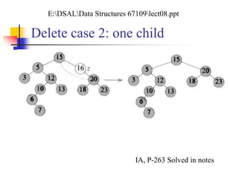
if x has two children (subtrees) case 2
then swap x with its successor
perform case 0 or case 1 to delete it
TOTAL: O(h) time to delete a node](https://image.slidesharecdn.com/chapter9ds-190904110931/85/Chapter-9-ds-25-320.jpg)
![Deletion – Pseudocode (1/2)
Tree-Delete(T, z)
/* Determine which node to splice out: either z or z’s successor. */
if left[z] = NIL or right[z] = NIL
then y z
else y Tree-Successor[z]
/* Set x to a non-NIL child of x, or to NIL if y has no children. */
4. if left[y] NIL
5. then x left[y]
6. else x right[y]
/* y is removed from the tree by manipulating pointers of p[y] and x */
7. if x NIL
8. then p[x] p[y]
/* Continued on next slide */](https://image.slidesharecdn.com/chapter9ds-190904110931/85/Chapter-9-ds-26-320.jpg)
![Deletion – Pseudocode (2/2)
Tree-Delete(T, z) (Contd. from previous slide)
9. if p[y] = NIL
10. then root[T] x
11. else if y left[p[i]]
12. then left[p[y]] x
13. else right[p[y]] x
/* If z’s successor was spliced out, copy its data into z */
14. if y z
15. then key[z] key[y]
16. copy y’s satellite data into z.
17. return y](https://image.slidesharecdn.com/chapter9ds-190904110931/85/Chapter-9-ds-27-320.jpg)

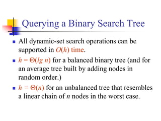
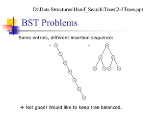
![Inefficiency of general BSTs
All operations in BST are performed in time
O(h), where h is the height of BST
Unfortunately h might be as large as n, e.g.,
after n consecutive insertions of elements with
keys in increasing order
The advantages of the binary search (O(log n)
time update) might be lost if BST is not
balanced
E:DSALcomp202 ULPweek3[1].ppt](https://image.slidesharecdn.com/chapter9ds-190904110931/85/Chapter-9-ds-31-320.jpg)
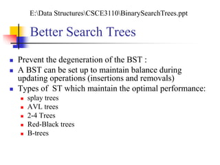

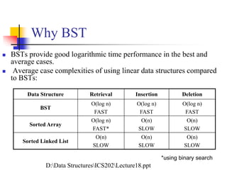
The document discusses binary search trees (BSTs), including their representation as linked data structures, common operations like search, insertion, deletion, finding minimum/maximum elements, and predecessors/successors. While BST operations take O(h) time where h is the tree height, h can be as large as n for an unbalanced tree. The document thus notes that better balanced search trees like AVL trees and red-black trees are preferable to ensure O(log n) performance of operations.