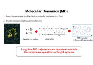
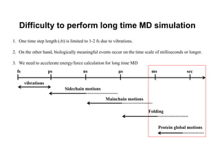
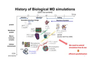
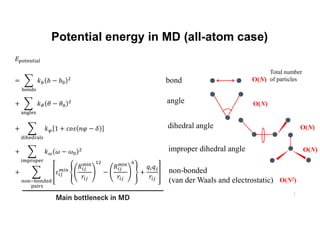
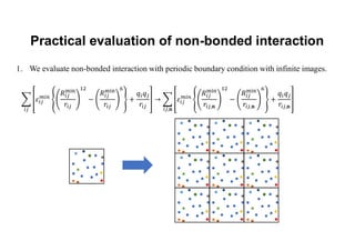
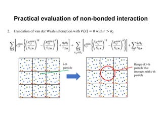
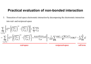
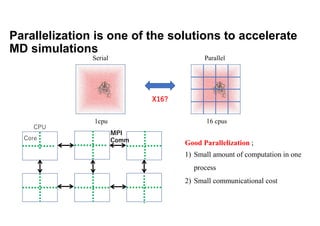
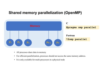
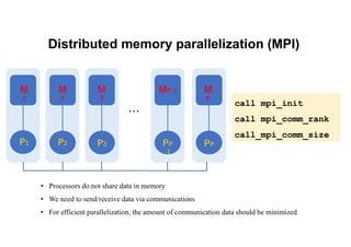
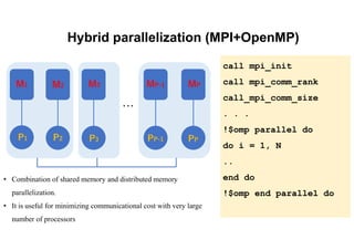
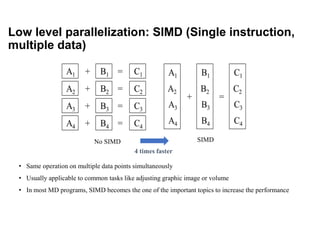
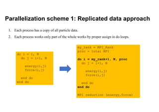
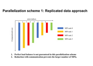
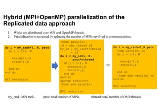
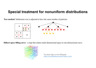
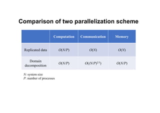
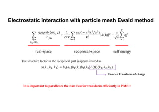
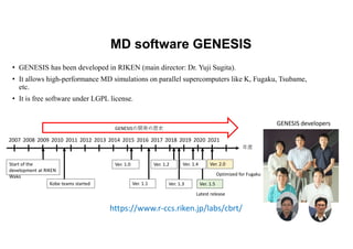
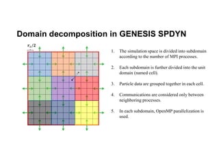
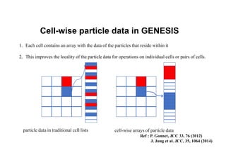
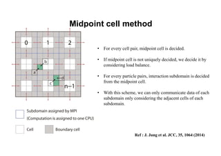
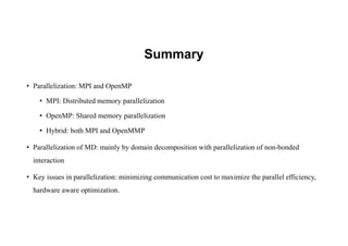
Parallelization of molecular dynamics
計算科学技術特論A
2021年 7月 8日
Jaewoon Jung
(RIKEN Center for Computational Science)
Overview of MD
Molecular Dynamics (MD)
1. Energy/forces are described by classical molecular mechanics force field.
2. Update state according to equations of motion
Long time MD trajectories are important to obtain
thermodynamic quantities of target systems.
Equation of motion
MD trajectory
=> Ensemble generation
Integration
𝐩 𝑡 +
1
2
∆𝑡 = 𝐩 𝑡 −
1
2
∆𝑡 + 𝐅 𝑡 ∆𝑡
𝐫 𝑡 + ∆𝑡 = 𝐫 𝑡 +
𝐩 𝑡 +
1
2
∆𝑡 ∆𝑡
𝑚
MD integration (Velocity Verlet case)
𝑡 +
1
2
∆𝑡 𝑡 + ∆𝑡 𝑡 +3∆𝑡
𝑡 +
5
2
∆𝑡
𝑡 +
3
2
∆𝑡
𝑡
coordinate update
𝐪 𝑡 → 𝐪 𝑡 + ∆𝑡
𝐩 𝑡 +
1
2
∆𝑡
→ 𝐩 𝑡 + ∆𝑡
coordinate update
𝐪 𝑡 + ∆𝑡 → 𝐪 𝑡 + 2∆𝑡
𝑡 + 2∆𝑡
coordinate update
𝐪 𝑡 + 2∆𝑡 → 𝐪 𝑡 + 3∆𝑡
𝐩 𝑡
→ 𝐩 𝑡 +
1
2
∆𝑡
𝐩 𝑡 + ∆𝑡
→ 𝐩 𝑡 +
3
2
∆𝑡
𝐩 𝑡 +
3
2
∆𝑡
→ 𝐩 𝑡 + 2∆𝑡
𝐩 𝑡 + 2∆𝑡
→ 𝐩 𝑡 +
5
2
∆𝑡
𝐩 𝑡 +
5
2
∆𝑡
→ 𝐩 𝑡 + 3∆𝑡
𝐅(𝑡) 𝐅(𝑡 + 2∆𝑡)
𝐅(𝑡 + ∆𝑡) 𝐅(𝑡 + 3∆𝑡)
Difficulty to perform long time MD simulation
1. One time step length (Δt) is limited to 1-2 fs due to vibrations.
2. On the other hand, biologically meaningful events occur on the time scale of milliseconds or longer.
3. We need to accelerate energy/force calculation for long time MD
fs ps ns μs ms sec
vibrations
Sidechain motions
Mainchain motions
Folding
Protein global motions
History of Biological MD simulations
(1977 to current)
ps ns ms ms s
vibration
Membrane
protein
Macro-
molecule
complex
size
(# of atoms)
Ribosome
(~2x10⁶) 2013
BPTI
(~6x10²)
1977
AQP1
(~105) 2000 BPTI, Ubiquitin
(~2x10⁴)
Mycoplasma
genitalium
(~1.0x10⁸)
HIV-1 capsid
(~6.5x10⁷)
ANTON
(Gordon Bell Prize 2009)
Chromatin
(~1.0x10⁹)
HIV-1 capsid
(~6.5x10⁷)
HP36
(~104)
KNL
Chromatophor
e vesicle
(~1.4x10⁸)
protein
Cellular
environment We need to extend
simulation time & size
time
relaxation folding
Reaction of protein
Secondary structure change
~2019
efficient parallelization
6
Potential energy in MD (all-atom case)
7
O(N)
O(N)
O(N)
O(N2)
Main bottleneck in MD
Total number
of particles
bond
angle
dihedral angle
improper dihedral angle
non-bonded
(van der Waals and electrostatic)
O(N)
Practical evaluation of non-bonded interaction
1. We evaluate non-bonded interaction with periodic boundary condition with infinite images.
,𝐧 ,𝐧 ,𝐧
,𝐧
Practical evaluation of non-bonded interaction
2. Truncation of van der Waals interaction with with
,𝐧 ,𝐧 ,𝐧
,𝐧 ,𝐧 ,𝐧
,𝐧 ,𝐧
i-th
particle
Range of j-th
particle that
interacts with i-th
particle
Practical evaluation of non-bonded interaction
3. Truncation of real-space electrostatic interaction by decomposing the electrostatic interaction
into real- and reciprocal-space
,𝐧 ,𝐧
,𝐧 ,𝐧
,𝐧 ,𝐧
,𝐧
,𝐧
,𝐧 𝐤 𝟎
real-space reciprocal-space self term
Parallelization is one of the solutions to accelerate
MD simulations
Serial Parallel
16 cpus
X16?
1cpu
1cpu
Good Parallelization ;
1) Small amount of computation in one
process
2) Small communicational cost
C
CPU
Core
MPI
Comm
Parallelization
Shared memory parallelization (OpenMP)
Memory
P1 P2 P3 PP-1 PP
• All processes share data in memory
• For efficient parallelization, processes should not access the same memory address.
• It is only available for multi-processors in a physical node
#pragma omp parallel
!$omp parallel
C
Fortran
Distributed memory parallelization (MPI)
M
1
P1
M
2
P2
M
3
P3
MP-1
PP
-1
M
P
PP
…
• Processors do not share data in memory
• We need to send/receive data via communications
• For efficient parallelization, the amount of communication data should be minimized
call mpi_init
call mpi_comm_rank
call_mpi_comm_size
Hybrid parallelization (MPI+OpenMP)
M1
P1
M2
P2
M3
P3
MP-1
PP-1
MP
PP
…
• Combination of shared memory and distributed memory
parallelization.
• It is useful for minimizing communicational cost with very large
number of processors
call mpi_init
call mpi_comm_rank
call_mpi_comm_size
. . .
!$omp parallel do
do i = 1, N
..
end do
!$omp end parallel do
Low level parallelization: SIMD (Single instruction,
multiple data)
• Same operation on multiple data points simultaneously
• Usually applicable to common tasks like adjusting graphic image or volume
• In most MD programs, SIMD becomes the one of the important topics to increase the performance
SIMD
No SIMD
4 times faster
MPI Parallelization of MD
(non-bonded interaction in real space)
Parallelization scheme 1: Replicated data approach
1. Each process has a copy of all particle data.
2. Each process works only part of the whole works by proper assign in do loops.
do i = 1, N
do j = i+1, N
energy(i,j)
force(i,j)
end do
end do
my_rank = MPI_Rank
proc = total MPI
do i = my_rank+1, N, proc
do j = i+1, N
energy(i,j)
force(i,j)
end do
end do
MPI reduction (energy,force)
MPI rank 1
MPI rank 0
MPI rank 2
MPI rank 3
atom indices
Computational
cost
1 2 3 4 5 6 7 8
1. Perfect load balance is not guaranteed in this parallelization scheme
2. Reduction with communication prevents the larger number of MPIs.
Parallelization scheme 1: Replicated data approach
Hybrid (MPI+OpenMP) parallelization of the
Replicated data approach
1. Works are distributed over MPI and OpenMP threads.
2. Parallelization is increased by reducing the number of MPIs involved in communications.
do i = my_rank+1, N, proc
do j = i+1, N
energy(i,j)
force(i,j)
end do
end do
MPI reduction
!$omp parallel
id = omp thread id
my_id = my_rank*nthread
+ id
do i = my_id+1, N,
proc*nthread
do j = i+1, N
energy(i,j)
force(i,j)
end do
end do
Openmp reduciton
!$omp end parallel
MPI reduction
do i = my_rank+1,N,proc
!omp parallel do
do j = i+1, N
energy(i,j)
force(i,j)
end do
!$omp end parallel do
end do
MPI reduction
my_rank: MPI rank, proc: total number of MPIs, nthread: total number of OMP threads
or
Pros and Cons of the Replicated data approach
1. Pros : easy to implement
2. Cons
• Parallel efficiency is not good
• No perfect load balance
• Communication cost is not reduced by increasing the number of processes
• We can parallelize only for energy calculation (with MPI, parallelization of integration is
not so much efficient)
• Needs a lot of memory
• Usage of global data
Parallelization scheme 2: Domain decomposition
1. The simulation space is divided into
subdomains according to MPI (different
colors for different MPIs).
2. Each MPI only considers the
corresponding subdomain.
3. MPI communications only among
neighboring processes.
Communications
between processors
Parallelization scheme 2: Domain decomposition
1. For the interaction between different subdomains, it
is necessary to have the data of the buffer region of
each subdomain.
2. The size of the buffer region is dependent on the
cutoff values.
3. The interaction between particles in different
subdomains should be considered very carefully.
4. The size of the subdomain and buffer region is
decreased by increasing the number of processes.
𝒓𝒄
Sub-
domain
Buffer
Pros and Cons of the domain decomposition approach
1. Pros
• Good parallel efficiency
• Reduced computational cost by increasing the number of processes
• We can easily parallelize not only energy but also integration
• Availability of a huge system
• Data size is decreased by increasing the number of processes
2. Cons
• Implementation is not easy
• Domain decomposition scheme is highly depend on the potential energy type, cutoff and so
on
• Good performance cannot be obtained for nonuniform particle distributions
Special treatment for nonuniform distributions
Tree method: Subdomain size is adjusted to have the same number of particles
Hilbert space filling curve : a map that relates multi-dimensional space to one-dimensional curve
The above figure is from Wikipedia
https://en.wikipedia.org/wiki/Hilbert_curve
Comparison of two parallelization scheme
Computation Communication Memory
Replicated data O(N/P) O(N) O(N)
Domain
decomposition
O(N/P) O((N/P)2/3) O(N/P)
N: system size
P: number of processes
MPI Parallelization of MD
(reciprocal space)
Electrostatic interaction with particle mesh Ewald method
real-space reciprocal-space self energy
The structure factor in the reciprocal part is approximated as
Fourier Transform of charge
It is important to parallelize the Fast Fourier transform efficiently in PME!!
,𝐧
,𝐧
,𝐧 𝐤 𝟎
Overall procedure of reciprocal space calculation
(charge on real space) (charge on grid)
Energy calculation
Force calculation
from
FFT
Inverse
FFT
Simple note of MPI_alltoall communications
MPI_alltoall
A1
A3
A2
B1
A4
B2
B4
B3
C2
C1
C3
C4
D1
D2
D4
D3
Proc1 Proc2 Proc3 Proc4
A1
C1
B1
A2
D1
B2
D2
C2
B3
A3
C3
D3
A4
B4
D4
C4
Proc1 Proc2 Proc3 Proc4
MPI_alltoall is same as matrix transpose!!
Parallel 3D FFT – slab (1D) decomposition
1. Each process is assigned a slab of size
for computing FFT of grids
on processes.
2. The scalability is limited by
3. should be divisible by
Parallel 3D FFT – slab (1D) decomposition
No
communication
MPI_Alltoall
communication among all
preocessors
Parallel 3D FFT – slab (1D) decomposition
1. Slab decomposition of 3D FFT has three steps
• 2D FFT (or two 1D FFT) along the two local dimension
• Global transpose (communication)
• 1D FFT along third dimension
2. Pros
• fast using small number of processes
3. Cons
• Limitation of the number of processes
Parallel 3D FFT –2D decomposition
MPI_Alltoall communications
among 3 processes of the same
color
MPI_Alltoall communications
among 3 processes of the same
color
Parallel 3D FFT –2D decomposition
1. 2D decomposition of 3D FFT has five steps
• 1D FFT along the local dimension
• Global transpose
• 1D FFT along the second dimension
• Global transpose
• 1D FFT along the third dimension
2. The global transpose requires communication only between subgroups of all
nodes
3. Cons: Slower than 1D decomposition for a small number of processes
4. Pros : Maximum parallelization is increased
Parallel 3D FFT – 3D decomposition
• More communications than existing FFT
• MPI_Alltoall communications only in
one dimensional space
• Reduce communicational cost for large
number of processes
Ref) J. Jung et al. Comput. Phys. Comm. 200, 57-65 (2016)
Case Study:
Parallelization in GENESIS MD software on Fugaku
supercomputer
MD software GENESIS
• GENESIS has been developed in RIKEN (main director: Dr. Yuji Sugita).
• It allows high-performance MD simulations on parallel supercomputers like K, Fugaku, Tsubame,
etc.
• It is free software under LGPL license.
年度
GENESISの開発の歴史
Start of the
development at RIKEN
Wako
Kobe teams started
Ver. 1.0
Ver. 1.1
2009 2010 2015 2016
Ver. 1.2
Ver. 1.3
2018 2019
2007 2008 2011 2012 2013 2014 2017 2020 2021
Ver. 1.5
Ver. 1.4 Ver. 2.0
Latest release
Optimized for Fugaku
https://www.r-ccs.riken.jp/labs/cbrt/
GENESIS developers
Domain decomposition in GENESIS SPDYN
1. The simulation space is divided into subdomain
according to the number of MPI processes.
2. Each subdomain is further divided into the unit
domain (named cell).
3. Particle data are grouped together in each cell.
4. Communications are considered only between
neighboring processes.
5. In each subdomain, OpenMP parallelization is
used.
𝒓𝒄/𝟐
Cell-wise particle data in GENESIS
1. Each cell contains an array with the data of the particles that reside within it
2. This improves the locality of the particle data for operations on individual cells or pairs of cells.
particle data in traditional cell lists
Ref : P. Gonnet, JCC 33, 76 (2012)
J. Jung et al. JCC, 35, 1064 (2014)
cell-wise arrays of particle data
Midpoint cell method
• For every cell pair, midpoint cell is decided.
• If midpoint cell is not uniquely decided, we decide it by
considering load balance.
• For every particle pairs, interaction subdomain is decided
from the midpoint cell.
• With this scheme, we can only communicate data of each
subdomain only considering the adjacent cells of each
subdomain.
Ref : J. Jung et al. JCC, 35, 1064 (2014)
Subdomain structure with midpoint cell method
1. Each MPI has local subdomain which is surrounded by boundary cells.
2. At least, the local subdomain has at least two cells in each direction
Local sub-domain
Boundary
𝑟 /2
Hybrid Parallelization of GENESIS (real-space)
Unit cell
Subdomain of each MPI
1 2
3 4
6
5 7 8
9 10
13
11
14
12
15 16
Cell pair Midpoint cell?
(1,1) Yes
(2,2) Yes
… …
(1,2) Yes
(1,3) Yes
… …
(1,5) Yes
(1,6) No
(1,7) No
(1,8) Yes
(1,9) No
(1,10) Yes
… …
thread1
thread4
thread4
thread3
thread1
thread2
thread2
OpenMP
parallelization
The parallelization scheme is changed on Fugaku for higher speed!!
Previous non-boned interaction scheme for K
Sign of atom pairs within pairlist cutoff distance
(3)
(4)
(4)
(4)
(6)
(5)
(4)
(3)
do ijcel = 1, ncell_pair
icel = cell_pair(ijcel)
jcel = cell_pair(ijcel)
do ix = 1, natom(icel)
do k = 1, nb15(ix,ijcel)
jx = nb15_list(k,ix,ijcel)
dij(1:3) = coord(1:3,ix,icel)
- coord(1:3,jx,jcel)
. . .
force calculation
end do
end do
end do
first cell index
second cell index
index of the first cell
index of the second cell
Fugaku supercomputer
1. Number of Nodes: 158,976
2. Each node has 4 core memory groups (CMGs)
3. Each CMG has 12 cores with 2.0 GHz clock speed
4. In each node, there are assistant cores (2 cores for computational node and 4 cores for I/O
and computational node)
5. HBM 32 GiB memory
6. Tofu Interconnect D
7. 16 SIMD widths with single precision
8. Peak performance: 488 Petalflops with double precision
How to optimize on Fugaku?
1. In principle, there is no difference between Algorithm1 and Algorithm2 because of the same operation
amount.
2. On Fugaku, Algorithm2 has better performance than Algorithm1.
3. The main reason is the operand waiting time for each do loop. On Fugaku, there are nonnegligible waiting
time before executing calculations in the do loop.
4. To minimize the waiting time, the most inner do loop length should be long.
5. If the most inner do loop length is small, it would be better not to vectorize when compiling.
do ij = 1, 256
index i and j from ij
f(i,j)
end do
end do
do i = 1, 16
do j = 1, 16
f(i,j)
end do
end do
Algorithm2 (O)
Algorithm1 (X)
do i = 1, 3
f(i)
end do
!$ocl nosimd
do i = 1, 3
f(i)
end do
f(1:3)
!$ocl nosimd
f(1:3)
f(1), f(2), f(3)
Nonbond interaction scheme on Fugaku :
New coordinate array
1 2 3 4 5 6 7 8 9 10 1 2 3 4 5 6 7 8 9 10 1 2 3 4 5 6 7 8 9 10 …
1st cell 3rd cell
2nd cell
1 2 3 4 5 6 7 8 9 10 11 12 13 14 15 16 17 18 19 20 21 22 23 24 25 26 27 28 29 30 …
coord_pbc(1:3,1:MaxAtom,1:ncel) → coord_pbc(1:3,1:MaxAtom×ncell)
Non-bonded interaction scheme on Fugaku
48
1
2
3
4
5
6
7
8
1 2 3 4 5 6 7 8
1
2
3
4
5
6
7
8
1 2 3 4 5 6 7 8
1
2
3
4
5
6
7
8
1 2 3 4 5 6
1
2
3
4
5
6
7
8
1 2 3 4 5 6 7 8 9
(1,2) cell pair (1,5) cell pair
(1,4) cell pair
(1,3) cell pair
1
2
3
4
5
6
7
8
1 2 3 4 5 6 7 8 1112 16 21 22 2931 38
. . .
. . . . . .
Large do
loop length
11 12 13 14 15 16 21 22 23 24 25 26 27 28 29 31 32 33 34 35 36 37 38
(15)
(15)
(15)
(14)
(19)
(17)
(15)
(9)
Nonbond interaction scheme on Fugaku
(Pseudo code)
do icel = 1, ncell
do ix = 1, natom(icel)
i = (icel-1)*MaxAtom + ix
rtmp(1:3) = coord(1:3,i)
do k = 1, nb15(ix,i)
j = nb15_list(k,ix,i)
dij(1:3) = rtmp(1:3)-coord(1:3,j)
. . .
force calculation
end do
Larger do loop length than K or Generic kernel
i is same as (ix,icel)
Comparison of non-bonded algorithms
do ijcel = 1, cell_pair
obtain icel and jcel
do i=1,natom(icel)
do k=1,neighbor(i,ijcel)
j = list(k,ijcel)
interaction end do
end do
end do
do icel = 1, cell
do i=1,natom(icel)
do k=1,neighbor(i,icel)
list(k,i,icel)
interaction end do
end do
end do
ApoA1 on one MPI processor
K Fugaku
prefetch
Prefetch is a technique used by computer processors to boost execution performance by fetching
instructions or data from their original storage in slower memory to a faster local memory before it is
actually needed (from Wikipedia).
Overall procedure of reciprocal-space interaction
(charge in real space) (charge grid data)
E( )
Force from
PME_Pre
FFT
Inverse FFT
PME_Post
Charge grid data evaluation in GENESIS 1.X
grids
1.Charge values is transferred to the neighbor grids.
2.The amount of neighbor depends on the spline order.
Real-space Reciprocal-space
Generated
charge grid
Accepted
charge grid
In this scheme, we can avoid communication in charge grid data generation.
Problem of charge grid data in GENESIS 1.X
Real-space Reciprocal-space
?
• We assume that charge grids in reciprocal-space is obtained from the real-space subdomain and its adjacent
cells.
• If the spline order and grid spacing is large (e.g. spline order 8 with grid spacing 2Å), the charge data of
adjacent cell is not sufficient to obtain the charge grid data in the subdomain.
New scheme of charge grid data for Fugaku (1)
Real-space Reciprocal-space
• Charge grid data is obtained from the charge values in the subdomain only.
• In this way, we don’t have to consider charge grid data loss even for large spline order.
New scheme of charge grid data for Fugaku (2)
Real-space Reciprocal-space
1. In the new scheme, we generate charge grid
data only from the subdomain.
2. Charge grid data generated out of the
subdomain is sent to next subdomain with
communication.
3. It accelerates the speed by reducing
operation and higher order spline can be
used.
4. The communication used is not global, so it
does not lose the performance significantly.
Real-space non-bonded interaction
(performance per node)
Algorithm 2 Algorithm 3
Time/step 26.99 ms 10.08 ms
FLOPS 18.91 GFLOPS 46.16 GFLOPS
Waiting time/step 18.43 ms 6.23 ms
Force calculation
Pairlist generation
Algorithm 2 Algorithm 3
Time/cycle 41.46 ms 17.56 ms
FLOPS 14.32 GFLOPS 33.58 GFLOPS
Waiting time/cycle 18.60 ms 8.65 ms
• Target system: 1.58 million atom system on 16 nodes
• 12.0 Å cutoff and 13.5 Å pairlist cutoff
Reciprocal-space non-bonded interaction
1. The new scheme increases the performance for small number of processors.
2. The new scheme also increases the overall performance by reducing grid numbers while increasing
spline order.
Node #
PME_new_3d PME_old_3d PME_new_2d PME_old_2d
1Åa 2 Åb 1Åa 1Åa 2 Åb 1Åa
256 57.3 38.4 61.7 46.6 38.1 52.6
512 27.6 20.2 29.5 29.4 20.8 32.3
1024 18.7 11.7 18.8 19.0 12.2 19.5
2048 13.9 6.9 13.5 17.5 7.4 17.1
4096 9.5 4.8 8.7 14.5 N/A 13.6
a Grid spacing is 1 Å, spline order is 4, and grid numbers are 1024×1024×1024
b Grid spacing is 2 Å, spline order is 8, and grid numbers are 512×512×512
• Target system: 101.12 million atoms
• 3d: 3D FFT decomposition
• 2d: 2D FFT decomposition
Conventional MD (weak scaling)
Number of nodes System size
grid spacing
= 1 Å
grid spacing
= 2 Å
16 1.58 M 11.62 (1.00) 11.29 (1.00)
32 3.16 M 11.12 (0.96) 11.11 (0.98)
64 6.32 M 11.07 (0.95) 11.10 (0.98)
128 12.63 M 10.82 (0.93) 10.99 (0.97)
256 25.26 M 10.01 (0.86) 10.72 (0.95)
512 50.53 M 10.27 (0.88) 10.82 (0.96)
1024 101.05 M 9.26 (0.80) 10.43 (0.92)
2048 202.11 M 8.53 (0.73) 10.26 (0.91)
4096 404.21 M 7.54 (0.65) 9.92 (0.88)
8192 808.43 M 7.23 (0.62) 9.13 (0.81)
16384 1.62 B 6.19 (0.53) 8.30 (0.74)
• Numbers in parentheses are weak scaling efficiency.
• By reducing grid numbers while increasing spline order, we can increase the performance for larger number of
nodes.
• We obtained best performance of the largest system (1.62B system with 8.30 ns/day) that is better than
existing (NAMD on Titan is 1B system with 5 ns/day).
Conventional MD (strong scaling)
11.9 ns/day
(more than twice better
performance than NAMD)
4 times better performance
than GENESIS1.0 on K using
1/8 nodes
Summary
• Parallelization: MPI and OpenMP
• MPI: Distributed memory parallelization
• OpenMP: Shared memory parallelization
• Hybrid: both MPI and OpenMMP
• Parallelization of MD: mainly by domain decomposition with parallelization of non-bonded
interaction
• Key issues in parallelization: minimizing communication cost to maximize the parallel efficiency,
hardware aware optimization.

第13回 配信講義 計算科学技術特論A(2021)

  • 1.
    Parallelization of moleculardynamics 計算科学技術特論A 2021年 7月 8日 Jaewoon Jung (RIKEN Center for Computational Science)
  • 2.
  • 3.
    Molecular Dynamics (MD) 1.Energy/forces are described by classical molecular mechanics force field. 2. Update state according to equations of motion Long time MD trajectories are important to obtain thermodynamic quantities of target systems. Equation of motion MD trajectory => Ensemble generation Integration 𝐩 𝑡 + 1 2 ∆𝑡 = 𝐩 𝑡 − 1 2 ∆𝑡 + 𝐅 𝑡 ∆𝑡 𝐫 𝑡 + ∆𝑡 = 𝐫 𝑡 + 𝐩 𝑡 + 1 2 ∆𝑡 ∆𝑡 𝑚
  • 4.
    MD integration (VelocityVerlet case) 𝑡 + 1 2 ∆𝑡 𝑡 + ∆𝑡 𝑡 +3∆𝑡 𝑡 + 5 2 ∆𝑡 𝑡 + 3 2 ∆𝑡 𝑡 coordinate update 𝐪 𝑡 → 𝐪 𝑡 + ∆𝑡 𝐩 𝑡 + 1 2 ∆𝑡 → 𝐩 𝑡 + ∆𝑡 coordinate update 𝐪 𝑡 + ∆𝑡 → 𝐪 𝑡 + 2∆𝑡 𝑡 + 2∆𝑡 coordinate update 𝐪 𝑡 + 2∆𝑡 → 𝐪 𝑡 + 3∆𝑡 𝐩 𝑡 → 𝐩 𝑡 + 1 2 ∆𝑡 𝐩 𝑡 + ∆𝑡 → 𝐩 𝑡 + 3 2 ∆𝑡 𝐩 𝑡 + 3 2 ∆𝑡 → 𝐩 𝑡 + 2∆𝑡 𝐩 𝑡 + 2∆𝑡 → 𝐩 𝑡 + 5 2 ∆𝑡 𝐩 𝑡 + 5 2 ∆𝑡 → 𝐩 𝑡 + 3∆𝑡 𝐅(𝑡) 𝐅(𝑡 + 2∆𝑡) 𝐅(𝑡 + ∆𝑡) 𝐅(𝑡 + 3∆𝑡)
  • 5.
    Difficulty to performlong time MD simulation 1. One time step length (Δt) is limited to 1-2 fs due to vibrations. 2. On the other hand, biologically meaningful events occur on the time scale of milliseconds or longer. 3. We need to accelerate energy/force calculation for long time MD fs ps ns μs ms sec vibrations Sidechain motions Mainchain motions Folding Protein global motions
  • 6.
    History of BiologicalMD simulations (1977 to current) ps ns ms ms s vibration Membrane protein Macro- molecule complex size (# of atoms) Ribosome (~2x10⁶) 2013 BPTI (~6x10²) 1977 AQP1 (~105) 2000 BPTI, Ubiquitin (~2x10⁴) Mycoplasma genitalium (~1.0x10⁸) HIV-1 capsid (~6.5x10⁷) ANTON (Gordon Bell Prize 2009) Chromatin (~1.0x10⁹) HIV-1 capsid (~6.5x10⁷) HP36 (~104) KNL Chromatophor e vesicle (~1.4x10⁸) protein Cellular environment We need to extend simulation time & size time relaxation folding Reaction of protein Secondary structure change ~2019 efficient parallelization 6
  • 7.
    Potential energy inMD (all-atom case) 7 O(N) O(N) O(N) O(N2) Main bottleneck in MD Total number of particles bond angle dihedral angle improper dihedral angle non-bonded (van der Waals and electrostatic) O(N)
  • 8.
    Practical evaluation ofnon-bonded interaction 1. We evaluate non-bonded interaction with periodic boundary condition with infinite images. ,𝐧 ,𝐧 ,𝐧 ,𝐧
  • 9.
    Practical evaluation ofnon-bonded interaction 2. Truncation of van der Waals interaction with with ,𝐧 ,𝐧 ,𝐧 ,𝐧 ,𝐧 ,𝐧 ,𝐧 ,𝐧 i-th particle Range of j-th particle that interacts with i-th particle
  • 10.
    Practical evaluation ofnon-bonded interaction 3. Truncation of real-space electrostatic interaction by decomposing the electrostatic interaction into real- and reciprocal-space ,𝐧 ,𝐧 ,𝐧 ,𝐧 ,𝐧 ,𝐧 ,𝐧 ,𝐧 ,𝐧 𝐤 𝟎 real-space reciprocal-space self term
  • 11.
    Parallelization is oneof the solutions to accelerate MD simulations Serial Parallel 16 cpus X16? 1cpu 1cpu Good Parallelization ; 1) Small amount of computation in one process 2) Small communicational cost C CPU Core MPI Comm
  • 12.
  • 13.
    Shared memory parallelization(OpenMP) Memory P1 P2 P3 PP-1 PP • All processes share data in memory • For efficient parallelization, processes should not access the same memory address. • It is only available for multi-processors in a physical node #pragma omp parallel !$omp parallel C Fortran
  • 14.
    Distributed memory parallelization(MPI) M 1 P1 M 2 P2 M 3 P3 MP-1 PP -1 M P PP … • Processors do not share data in memory • We need to send/receive data via communications • For efficient parallelization, the amount of communication data should be minimized call mpi_init call mpi_comm_rank call_mpi_comm_size
  • 15.
    Hybrid parallelization (MPI+OpenMP) M1 P1 M2 P2 M3 P3 MP-1 PP-1 MP PP … •Combination of shared memory and distributed memory parallelization. • It is useful for minimizing communicational cost with very large number of processors call mpi_init call mpi_comm_rank call_mpi_comm_size . . . !$omp parallel do do i = 1, N .. end do !$omp end parallel do
  • 16.
    Low level parallelization:SIMD (Single instruction, multiple data) • Same operation on multiple data points simultaneously • Usually applicable to common tasks like adjusting graphic image or volume • In most MD programs, SIMD becomes the one of the important topics to increase the performance SIMD No SIMD 4 times faster
  • 17.
    MPI Parallelization ofMD (non-bonded interaction in real space)
  • 18.
    Parallelization scheme 1:Replicated data approach 1. Each process has a copy of all particle data. 2. Each process works only part of the whole works by proper assign in do loops. do i = 1, N do j = i+1, N energy(i,j) force(i,j) end do end do my_rank = MPI_Rank proc = total MPI do i = my_rank+1, N, proc do j = i+1, N energy(i,j) force(i,j) end do end do MPI reduction (energy,force)
  • 19.
    MPI rank 1 MPIrank 0 MPI rank 2 MPI rank 3 atom indices Computational cost 1 2 3 4 5 6 7 8 1. Perfect load balance is not guaranteed in this parallelization scheme 2. Reduction with communication prevents the larger number of MPIs. Parallelization scheme 1: Replicated data approach
  • 20.
    Hybrid (MPI+OpenMP) parallelizationof the Replicated data approach 1. Works are distributed over MPI and OpenMP threads. 2. Parallelization is increased by reducing the number of MPIs involved in communications. do i = my_rank+1, N, proc do j = i+1, N energy(i,j) force(i,j) end do end do MPI reduction !$omp parallel id = omp thread id my_id = my_rank*nthread + id do i = my_id+1, N, proc*nthread do j = i+1, N energy(i,j) force(i,j) end do end do Openmp reduciton !$omp end parallel MPI reduction do i = my_rank+1,N,proc !omp parallel do do j = i+1, N energy(i,j) force(i,j) end do !$omp end parallel do end do MPI reduction my_rank: MPI rank, proc: total number of MPIs, nthread: total number of OMP threads or
  • 21.
    Pros and Consof the Replicated data approach 1. Pros : easy to implement 2. Cons • Parallel efficiency is not good • No perfect load balance • Communication cost is not reduced by increasing the number of processes • We can parallelize only for energy calculation (with MPI, parallelization of integration is not so much efficient) • Needs a lot of memory • Usage of global data
  • 22.
    Parallelization scheme 2:Domain decomposition 1. The simulation space is divided into subdomains according to MPI (different colors for different MPIs). 2. Each MPI only considers the corresponding subdomain. 3. MPI communications only among neighboring processes. Communications between processors
  • 23.
    Parallelization scheme 2:Domain decomposition 1. For the interaction between different subdomains, it is necessary to have the data of the buffer region of each subdomain. 2. The size of the buffer region is dependent on the cutoff values. 3. The interaction between particles in different subdomains should be considered very carefully. 4. The size of the subdomain and buffer region is decreased by increasing the number of processes. 𝒓𝒄 Sub- domain Buffer
  • 24.
    Pros and Consof the domain decomposition approach 1. Pros • Good parallel efficiency • Reduced computational cost by increasing the number of processes • We can easily parallelize not only energy but also integration • Availability of a huge system • Data size is decreased by increasing the number of processes 2. Cons • Implementation is not easy • Domain decomposition scheme is highly depend on the potential energy type, cutoff and so on • Good performance cannot be obtained for nonuniform particle distributions
  • 25.
    Special treatment fornonuniform distributions Tree method: Subdomain size is adjusted to have the same number of particles Hilbert space filling curve : a map that relates multi-dimensional space to one-dimensional curve The above figure is from Wikipedia https://en.wikipedia.org/wiki/Hilbert_curve
  • 26.
    Comparison of twoparallelization scheme Computation Communication Memory Replicated data O(N/P) O(N) O(N) Domain decomposition O(N/P) O((N/P)2/3) O(N/P) N: system size P: number of processes
  • 27.
    MPI Parallelization ofMD (reciprocal space)
  • 28.
    Electrostatic interaction withparticle mesh Ewald method real-space reciprocal-space self energy The structure factor in the reciprocal part is approximated as Fourier Transform of charge It is important to parallelize the Fast Fourier transform efficiently in PME!! ,𝐧 ,𝐧 ,𝐧 𝐤 𝟎
  • 29.
    Overall procedure ofreciprocal space calculation (charge on real space) (charge on grid) Energy calculation Force calculation from FFT Inverse FFT
  • 30.
    Simple note ofMPI_alltoall communications MPI_alltoall A1 A3 A2 B1 A4 B2 B4 B3 C2 C1 C3 C4 D1 D2 D4 D3 Proc1 Proc2 Proc3 Proc4 A1 C1 B1 A2 D1 B2 D2 C2 B3 A3 C3 D3 A4 B4 D4 C4 Proc1 Proc2 Proc3 Proc4 MPI_alltoall is same as matrix transpose!!
  • 31.
    Parallel 3D FFT– slab (1D) decomposition 1. Each process is assigned a slab of size for computing FFT of grids on processes. 2. The scalability is limited by 3. should be divisible by
  • 32.
    Parallel 3D FFT– slab (1D) decomposition No communication MPI_Alltoall communication among all preocessors
  • 33.
    Parallel 3D FFT– slab (1D) decomposition 1. Slab decomposition of 3D FFT has three steps • 2D FFT (or two 1D FFT) along the two local dimension • Global transpose (communication) • 1D FFT along third dimension 2. Pros • fast using small number of processes 3. Cons • Limitation of the number of processes
  • 34.
    Parallel 3D FFT–2D decomposition MPI_Alltoall communications among 3 processes of the same color MPI_Alltoall communications among 3 processes of the same color
  • 35.
    Parallel 3D FFT–2D decomposition 1. 2D decomposition of 3D FFT has five steps • 1D FFT along the local dimension • Global transpose • 1D FFT along the second dimension • Global transpose • 1D FFT along the third dimension 2. The global transpose requires communication only between subgroups of all nodes 3. Cons: Slower than 1D decomposition for a small number of processes 4. Pros : Maximum parallelization is increased
  • 36.
    Parallel 3D FFT– 3D decomposition • More communications than existing FFT • MPI_Alltoall communications only in one dimensional space • Reduce communicational cost for large number of processes Ref) J. Jung et al. Comput. Phys. Comm. 200, 57-65 (2016)
  • 37.
    Case Study: Parallelization inGENESIS MD software on Fugaku supercomputer
  • 38.
    MD software GENESIS •GENESIS has been developed in RIKEN (main director: Dr. Yuji Sugita). • It allows high-performance MD simulations on parallel supercomputers like K, Fugaku, Tsubame, etc. • It is free software under LGPL license. 年度 GENESISの開発の歴史 Start of the development at RIKEN Wako Kobe teams started Ver. 1.0 Ver. 1.1 2009 2010 2015 2016 Ver. 1.2 Ver. 1.3 2018 2019 2007 2008 2011 2012 2013 2014 2017 2020 2021 Ver. 1.5 Ver. 1.4 Ver. 2.0 Latest release Optimized for Fugaku https://www.r-ccs.riken.jp/labs/cbrt/ GENESIS developers
  • 39.
    Domain decomposition inGENESIS SPDYN 1. The simulation space is divided into subdomain according to the number of MPI processes. 2. Each subdomain is further divided into the unit domain (named cell). 3. Particle data are grouped together in each cell. 4. Communications are considered only between neighboring processes. 5. In each subdomain, OpenMP parallelization is used. 𝒓𝒄/𝟐
  • 40.
    Cell-wise particle datain GENESIS 1. Each cell contains an array with the data of the particles that reside within it 2. This improves the locality of the particle data for operations on individual cells or pairs of cells. particle data in traditional cell lists Ref : P. Gonnet, JCC 33, 76 (2012) J. Jung et al. JCC, 35, 1064 (2014) cell-wise arrays of particle data
  • 41.
    Midpoint cell method •For every cell pair, midpoint cell is decided. • If midpoint cell is not uniquely decided, we decide it by considering load balance. • For every particle pairs, interaction subdomain is decided from the midpoint cell. • With this scheme, we can only communicate data of each subdomain only considering the adjacent cells of each subdomain. Ref : J. Jung et al. JCC, 35, 1064 (2014)
  • 42.
    Subdomain structure withmidpoint cell method 1. Each MPI has local subdomain which is surrounded by boundary cells. 2. At least, the local subdomain has at least two cells in each direction Local sub-domain Boundary 𝑟 /2
  • 43.
    Hybrid Parallelization ofGENESIS (real-space) Unit cell Subdomain of each MPI 1 2 3 4 6 5 7 8 9 10 13 11 14 12 15 16 Cell pair Midpoint cell? (1,1) Yes (2,2) Yes … … (1,2) Yes (1,3) Yes … … (1,5) Yes (1,6) No (1,7) No (1,8) Yes (1,9) No (1,10) Yes … … thread1 thread4 thread4 thread3 thread1 thread2 thread2 OpenMP parallelization The parallelization scheme is changed on Fugaku for higher speed!!
  • 44.
    Previous non-boned interactionscheme for K Sign of atom pairs within pairlist cutoff distance (3) (4) (4) (4) (6) (5) (4) (3) do ijcel = 1, ncell_pair icel = cell_pair(ijcel) jcel = cell_pair(ijcel) do ix = 1, natom(icel) do k = 1, nb15(ix,ijcel) jx = nb15_list(k,ix,ijcel) dij(1:3) = coord(1:3,ix,icel) - coord(1:3,jx,jcel) . . . force calculation end do end do end do first cell index second cell index index of the first cell index of the second cell
  • 45.
    Fugaku supercomputer 1. Numberof Nodes: 158,976 2. Each node has 4 core memory groups (CMGs) 3. Each CMG has 12 cores with 2.0 GHz clock speed 4. In each node, there are assistant cores (2 cores for computational node and 4 cores for I/O and computational node) 5. HBM 32 GiB memory 6. Tofu Interconnect D 7. 16 SIMD widths with single precision 8. Peak performance: 488 Petalflops with double precision
  • 46.
    How to optimizeon Fugaku? 1. In principle, there is no difference between Algorithm1 and Algorithm2 because of the same operation amount. 2. On Fugaku, Algorithm2 has better performance than Algorithm1. 3. The main reason is the operand waiting time for each do loop. On Fugaku, there are nonnegligible waiting time before executing calculations in the do loop. 4. To minimize the waiting time, the most inner do loop length should be long. 5. If the most inner do loop length is small, it would be better not to vectorize when compiling. do ij = 1, 256 index i and j from ij f(i,j) end do end do do i = 1, 16 do j = 1, 16 f(i,j) end do end do Algorithm2 (O) Algorithm1 (X) do i = 1, 3 f(i) end do !$ocl nosimd do i = 1, 3 f(i) end do f(1:3) !$ocl nosimd f(1:3) f(1), f(2), f(3)
  • 47.
    Nonbond interaction schemeon Fugaku : New coordinate array 1 2 3 4 5 6 7 8 9 10 1 2 3 4 5 6 7 8 9 10 1 2 3 4 5 6 7 8 9 10 … 1st cell 3rd cell 2nd cell 1 2 3 4 5 6 7 8 9 10 11 12 13 14 15 16 17 18 19 20 21 22 23 24 25 26 27 28 29 30 … coord_pbc(1:3,1:MaxAtom,1:ncel) → coord_pbc(1:3,1:MaxAtom×ncell)
  • 48.
    Non-bonded interaction schemeon Fugaku 48 1 2 3 4 5 6 7 8 1 2 3 4 5 6 7 8 1 2 3 4 5 6 7 8 1 2 3 4 5 6 7 8 1 2 3 4 5 6 7 8 1 2 3 4 5 6 1 2 3 4 5 6 7 8 1 2 3 4 5 6 7 8 9 (1,2) cell pair (1,5) cell pair (1,4) cell pair (1,3) cell pair 1 2 3 4 5 6 7 8 1 2 3 4 5 6 7 8 1112 16 21 22 2931 38 . . . . . . . . . Large do loop length 11 12 13 14 15 16 21 22 23 24 25 26 27 28 29 31 32 33 34 35 36 37 38 (15) (15) (15) (14) (19) (17) (15) (9)
  • 49.
    Nonbond interaction schemeon Fugaku (Pseudo code) do icel = 1, ncell do ix = 1, natom(icel) i = (icel-1)*MaxAtom + ix rtmp(1:3) = coord(1:3,i) do k = 1, nb15(ix,i) j = nb15_list(k,ix,i) dij(1:3) = rtmp(1:3)-coord(1:3,j) . . . force calculation end do Larger do loop length than K or Generic kernel i is same as (ix,icel)
  • 50.
    Comparison of non-bondedalgorithms do ijcel = 1, cell_pair obtain icel and jcel do i=1,natom(icel) do k=1,neighbor(i,ijcel) j = list(k,ijcel) interaction end do end do end do do icel = 1, cell do i=1,natom(icel) do k=1,neighbor(i,icel) list(k,i,icel) interaction end do end do end do ApoA1 on one MPI processor K Fugaku
  • 51.
    prefetch Prefetch is atechnique used by computer processors to boost execution performance by fetching instructions or data from their original storage in slower memory to a faster local memory before it is actually needed (from Wikipedia).
  • 52.
    Overall procedure ofreciprocal-space interaction (charge in real space) (charge grid data) E( ) Force from PME_Pre FFT Inverse FFT PME_Post
  • 53.
    Charge grid dataevaluation in GENESIS 1.X grids 1.Charge values is transferred to the neighbor grids. 2.The amount of neighbor depends on the spline order. Real-space Reciprocal-space Generated charge grid Accepted charge grid In this scheme, we can avoid communication in charge grid data generation.
  • 54.
    Problem of chargegrid data in GENESIS 1.X Real-space Reciprocal-space ? • We assume that charge grids in reciprocal-space is obtained from the real-space subdomain and its adjacent cells. • If the spline order and grid spacing is large (e.g. spline order 8 with grid spacing 2Å), the charge data of adjacent cell is not sufficient to obtain the charge grid data in the subdomain.
  • 55.
    New scheme ofcharge grid data for Fugaku (1) Real-space Reciprocal-space • Charge grid data is obtained from the charge values in the subdomain only. • In this way, we don’t have to consider charge grid data loss even for large spline order.
  • 56.
    New scheme ofcharge grid data for Fugaku (2) Real-space Reciprocal-space 1. In the new scheme, we generate charge grid data only from the subdomain. 2. Charge grid data generated out of the subdomain is sent to next subdomain with communication. 3. It accelerates the speed by reducing operation and higher order spline can be used. 4. The communication used is not global, so it does not lose the performance significantly.
  • 57.
    Real-space non-bonded interaction (performanceper node) Algorithm 2 Algorithm 3 Time/step 26.99 ms 10.08 ms FLOPS 18.91 GFLOPS 46.16 GFLOPS Waiting time/step 18.43 ms 6.23 ms Force calculation Pairlist generation Algorithm 2 Algorithm 3 Time/cycle 41.46 ms 17.56 ms FLOPS 14.32 GFLOPS 33.58 GFLOPS Waiting time/cycle 18.60 ms 8.65 ms • Target system: 1.58 million atom system on 16 nodes • 12.0 Å cutoff and 13.5 Å pairlist cutoff
  • 58.
    Reciprocal-space non-bonded interaction 1.The new scheme increases the performance for small number of processors. 2. The new scheme also increases the overall performance by reducing grid numbers while increasing spline order. Node # PME_new_3d PME_old_3d PME_new_2d PME_old_2d 1Åa 2 Åb 1Åa 1Åa 2 Åb 1Åa 256 57.3 38.4 61.7 46.6 38.1 52.6 512 27.6 20.2 29.5 29.4 20.8 32.3 1024 18.7 11.7 18.8 19.0 12.2 19.5 2048 13.9 6.9 13.5 17.5 7.4 17.1 4096 9.5 4.8 8.7 14.5 N/A 13.6 a Grid spacing is 1 Å, spline order is 4, and grid numbers are 1024×1024×1024 b Grid spacing is 2 Å, spline order is 8, and grid numbers are 512×512×512 • Target system: 101.12 million atoms • 3d: 3D FFT decomposition • 2d: 2D FFT decomposition
  • 59.
    Conventional MD (weakscaling) Number of nodes System size grid spacing = 1 Å grid spacing = 2 Å 16 1.58 M 11.62 (1.00) 11.29 (1.00) 32 3.16 M 11.12 (0.96) 11.11 (0.98) 64 6.32 M 11.07 (0.95) 11.10 (0.98) 128 12.63 M 10.82 (0.93) 10.99 (0.97) 256 25.26 M 10.01 (0.86) 10.72 (0.95) 512 50.53 M 10.27 (0.88) 10.82 (0.96) 1024 101.05 M 9.26 (0.80) 10.43 (0.92) 2048 202.11 M 8.53 (0.73) 10.26 (0.91) 4096 404.21 M 7.54 (0.65) 9.92 (0.88) 8192 808.43 M 7.23 (0.62) 9.13 (0.81) 16384 1.62 B 6.19 (0.53) 8.30 (0.74) • Numbers in parentheses are weak scaling efficiency. • By reducing grid numbers while increasing spline order, we can increase the performance for larger number of nodes. • We obtained best performance of the largest system (1.62B system with 8.30 ns/day) that is better than existing (NAMD on Titan is 1B system with 5 ns/day).
  • 60.
    Conventional MD (strongscaling) 11.9 ns/day (more than twice better performance than NAMD) 4 times better performance than GENESIS1.0 on K using 1/8 nodes
  • 61.
    Summary • Parallelization: MPIand OpenMP • MPI: Distributed memory parallelization • OpenMP: Shared memory parallelization • Hybrid: both MPI and OpenMMP • Parallelization of MD: mainly by domain decomposition with parallelization of non-bonded interaction • Key issues in parallelization: minimizing communication cost to maximize the parallel efficiency, hardware aware optimization.