Chapter 12 ds

Chapter 12
Hash Tables
Dr. Muhammad Hanif Durad
Department of Computer and Information Sciences
Pakistan Institute Engineering and Applied Sciences
hanif@pieas.edu.pk
Some slides have bee adapted with thanks from some other lectures
available on Internet. It made my life easier, as life is always
miserable at PIEAS (Sir Muhammad Yusaf Kakakhil )

Dr. Hanif Durad 2
Lecture Outline
 Hash Tables and their applications
 Common Hashing Functions
 Collision Resolution Techniques
 Separate Chaining
 Open-addressing
 Open-addressing
 Linear Probing
 Quadratic Probing
 Double Hashing
 Hashing Efficiency
 Rehashing

Hash Tables
 Recall order of magnitude of searches
 Linear search O(n)
 Binary search O(log2n)
 Balanced binary tree search O(log2n)
 Unbalanced binary tree can degrade to O(n)
E:Data StructuresHanif_SearchSearchingchapter12.ppt

Hash Tables
 In some situations faster search is needed
 Solution is to use a hash function
 Value of key field given to hash function
 Location in a hash table is calculated

Some Applications of Hash
Tables (1/2)
 Database systems: Specifically, those that require
efficient random access. Generally, database systems try
to optimize between two types of access methods:
sequential and random. Hash tables are an important part
of efficient random access because they provide a way to
locate data in a constant amount of time.
 Symbol tables: The tables used by compilers to maintain
information about symbols from a program. Compilers
access information about symbols frequently. Therefore, it
is important that symbol tables be implemented very
efficiently.
E:Data StructuresHanif_SearchSearching Unit28_Hashing1.ppt

 Data dictionaries: Data structures that support adding,
deleting, and searching for data. Although the operations
of a hash table and a data dictionary are similar, other
data structures may be used to implement data
dictionaries. Using a hash table is particularly efficient.
 Network processing algorithms: Hash tables are
fundamental components of several network processing
algorithms and applications, including route lookup,
packet classification, and network monitoring.
 Browser Cashes: Hash tables are used to implement
browser cashes.
Some Applications of Hash
Tables (2/2)

Example 1: Illustrating Hashing
(1/2)
 Use the function f(r) = r.id % 13 to load the following
records into an array of size 13.
9859261.73Zaid
9708761.60Musab
9809621.58Muneeb
9860741.80Adel
9707281.73Adnan
9945931.66Yousuf
9963211.70Husain

Example 1: Illustrating Hashing
(2/2)
0 1 2 3 4 5 6 7 8 9 10 11 12
h(r) = id % 13IDName
6985926Zaid
10970876Musab
8980962Muneeb
11986074Adel
5970728Adnan
2994593Yousuf
1996321Husain

Hash Tables (1/2)
 There are two types of Hash Tables:
 Open-addressed Hash Tables (closed hashing)
 Separate-Chained Hash Tables. (Open hashing)
 An Open-addressed Hash Table is a one-dimensional
array indexed by integer values that are computed by an
index function called a hash function.
 A Separate-Chained Hash Table is a one-dimensional
array of linked lists indexed by integer values that are
computed by an index function called a hash function.

Hash Tables (2/2)
 Hash tables are sometimes referred to as scatter
tables
 Typical hash table operations are:
1. Initialization.
2. Insertion.
3. Searching
4. Deletion.

Types of Hashing
 There are two types of hashing :
1. Static hashing: In static hashing, the hash function maps search-key values
to a fixed set of locations.
2. Dynamic hashing: In dynamic hashing a hash table can grow to handle more
items. The associated hash function must change as the table grows.
 The load factor of a hash table is the ratio of the number of keys in the table to
the size of the hash table.
 Note: The higher the load factor, the slower the retrieval.
 With open addressing (arrays) , the load factor cannot exceed 1. With chaining
(linked list ), the load factor often exceeds 1.

Hash Tables
 Constant time accesses!
 A hash table is an array of some
fixed size, usually a prime number.
 General idea:
key space (e.g., integers, strings)
0
…
TableSize –1
hash function:
h(K)
hash table
E:Data StructuresHanif_SearchSearchinghash.ppt

Hash Functions (1/2)
 A hash function, h, is a function which transforms a key from
a set, K, into an index in a table of size n:
h: K -> {0, 1, ..., n-2, n-1}
 A key can be a number, a string, a record etc.
 The size of the set of keys, |K|, to be relatively very large
(say m).
 It is possible for different keys to hash to the same array
location.
 This situation is called collision and the colliding keys are
called synonyms.

load factor -=m/n
m– number of elements in dictionary K
n – size of hash table
=m/n – load factor
(Note: 1)
Some text books define
With uniform hashing, a load factor of 0.5 means we
expect to find no more than two objects in one slot. For
load factors greater than 0.6 performance declines
dramatically.
E:Data StructuresHanif_SearchSearching hashing3.ppt, p-19/22
E:Data StructuresHanif_SearchSearching 12-3.ppt, p-13/16
=m/n – load factor
(Note: 1)

Hash Functions (2/2)
 A good hash function should:
 Minimize collisions.
 Be easy and quick to compute.
 Distribute key values evenly in the hash table.
 Use all the information provided in the key.

Common Hashing Functions
(1/6)
1. Division Remainder (using the table size as the divisor)
 Computes hash value from key using the % operator.
 Table size that is a power of 2 like 32 and 1024 should be avoided,
for it leads to more collisions.
 Also, powers of 10 are not good for table sizes when the keys rely
on decimal integers.
 Prime numbers not close to powers of 2 are better table size values.

2. Truncation or Digit/Character Extraction
 Works based on the distribution of digits or characters in the key.
 More evenly distributed digit positions are extracted and used for
hashing purposes.
 For instance, students IDs or ISBN codes may contain common
subsequences which may increase the likelihood of collision.
 Very fast but digits/characters distribution in keys may not be very
even.
(2/6)

3. Folding
 It involves splitting keys into two or more parts and then
combining the parts to form the hash addresses.
 To map the key 25936715 to a range between 0 and 9999, we
can:
 split the number into two as 2593 and 6715 and
 add these two to obtain 9308 as the hash value.
 Very useful if we have keys that are very large.
 Fast and simple especially with bit patterns.
A great advantage is ability to transform non-integer keys into
integer values.
(3/6)

4. Radix Conversion
 Transforms a key into another number base to obtain the hash
value.
 Typically use number base other than base 10 and base 2 to
calculate the hash addresses.
 To map the key 55354 in the range 0 to 9999 using base 11 we
have:
5535410 = 3865211
 We may truncate the high-order 3 to yield 8652 as our hash
address within 0 to 9999.
(4/6)

5. Mid-Square
 The key is squared and the middle part of the result taken as the
hash value.
 To map the key 3121 into a hash table of size 1000, we square it
31212 = 9740641 and extract 406 as the hash value.
 Works well if the keys do not contain a lot of leading or trailing
zeros.
 Non-integer keys have to be preprocessed to obtain corresponding
integer values.
(5/6)

6. Use of a Random-Number Generator
 Given a seed as parameter, the method generates a
random number.
 The algorithm must ensure that:
 It always generates the same random value for a given key.
 It is unlikely for two keys to yield the same random value.
 The random number produced can be transformed to
produce a valid hash value.
(6/6)

Problems for Which Hash Tables
are not Suitable (1/2)
1. Problems for which data ordering is required.
Because a hash table is an unordered data structure, certain
operations are difficult and expensive. Range queries, proximity
queries, selection, and sorted traversals are possible only if the
keys are copied into a sorted data structure. There are hash table
implementations that keep the keys in order, but they are far
from efficient.
2. Problems having multidimensional data.
3. Prefix searching especially if the keys are long and of variable-
lengths

Problems for Which Hash Tables
are not Suitable (1/2)
4. Problems that have dynamic data:
Open-addressed hash tables are based on 1D-arrays, which are
difficult to resize once they have been allocated. Unless you want to
implement the table as a dynamic array and rehash all of the keys
whenever the size changes. This is an incredibly expensive
operation. An alternative is use a separate-chained hash tables or
dynamic hashing.
5. Problems in which the data does not have unique keys.
Open-addressed hash tables cannot be used if the data does not have
unique keys. An alternative is use separate-chained hash tables

Hashing: Collision Resolution
Schemes
 Collision Resolution Techniques
 Separate Chaining
 Separate Chaining with String Keys
 Separate Chaining versus Open-addressing
 The class hierarchy of Hash Tables
 Implementation of Separate Chaining
 Introduction to Collision Resolution using Open
Addressing
 Linear Probing

Collision Resolution Techniques
 There are two broad ways of collision resolution:
1. Separate Chaining:: An array of linked list implementation.
2. Open Addressing: Array-based implementation.
(i) Linear probing (linear search)
(ii) Quadratic probing (nonlinear search)
(iii) Double hashing (uses two hash functions)

Separate Chaining (1/2)
• The hash table is implemented as an array of linked lists.
• Inserting an item, r, that hashes at index i is simply insertion into the linked list at
position i.
• Synonyms are chained in the same linked list.

Separate Chaining (2/2)
• Retrieval of an item, r, with hash address, i, is simply retrieval from the linked list
at position i.
• Deletion of an item, r, with hash address, i, is simply deleting r from the linked list
at position i.
• Example: Load the keys 23, 13, 21, 14, 7, 8, and 15 , in this order, in a hash table
of size 7 using separate chaining with the hash function: h(key) = key % 7
h(23) = 23 % 7 = 2
h(13) = 13 % 7 = 6
h(21) = 21 % 7 = 0
h(14) = 14 % 7 = 0 collision
h(7) = 7 % 7 = 0 collision
h(8) = 8 % 7 = 1
h(15) = 15 % 7 = 1 collision
unordered lists
ordered lists (?)
DS-1, P-518

Separate Chaining with String Keys (1/4)
• Recall that search keys can be numbers, strings or some other object.
• A hash function for a string s = c0c1c2…cn-1 can be defined as:
hash = (c0 + c1 + c2 + … + cn-1) % tableSize
this can be implemented as:
• Example: The following class describes commodity items:
public static int hash(String key, int tableSize){
int hashValue = 0;
for (int i = 0; i < key.length(); i++){
hashValue += key.charAt(i);
}
return hashValue % tableSize;
}
class CommodityItem {
String name; // commodity name
int quantity; // commodity quantity needed
double price; // commodity price
}

• Use the hash function hash to load the following commodity items into a
hash table of size 13 using separate chaining:
onion 1 10.0
tomato 1 8.50
cabbage 3 3.50
carrot 1 5.50
okra 1 6.50
mellon 2 10.0
potato 2 7.50
Banana 3 4.00
olive 2 15.0
salt 2 2.50
cucumber 3 4.50
mushroom 3 5.50
orange 2 3.00
• Solution:
hash(onion) = (111 + 110 + 105 + 111 + 110) % 13 = 547 % 13 = 1
hash(salt) = (115 + 97 + 108 + 116) % 13 = 436 % 13 = 7
hash(orange) = (111 + 114 + 97 + 110 + 103 + 101)%13 = 636 %13 = 12

0
1
2
3
4
5
6
7
8
9
10
11
12
onion
okra
mellon
banana
tomato olive
cucumber
mushroom
salt
cabbage
carrot
potato
orange
Item Qty Price h(key)
onion 1 10.0 1
tomato 1 8.50 10
cabbage 3 3.50 4
carrot 1 5.50 1
okra 1 6.50 0
mellon 2 10.0 10
potato 2 7.50 0
Banana 3 4.0 11
olive 2 15.0 10
salt 2 2.50 7
cucumber 3 4.50 9
mushroom 3 5.50 6
orange 2 3.00 12

Separate Chaining with String
Keys (4/4)
 Alternative hash functions for a string
s = c0c1c2…cn-1
exist, some are:
 hash = (c0 + 27 * c1 + 729 * c2) % tableSize
 hash = (c0 + cn-1 + s.length()) % tableSize

Separate Chaining versus Open-
addressing (1/2)
Separate Chaining has several advantages over open
addressing:
 Collision resolution is simple and efficient.
 The hash table can hold more elements without the large
performance deterioration of open addressing (The load factor
can be 1 or greater)
 The performance of chaining declines much more slowly than
open addressing.
 Deletion is easy - no special flag values are necessary.
 Table size need not be a prime number.
 The keys of the objects to be hashed need not be unique.

Separate Chaining versus Open-
addressing (1/2)
Disadvantages of Separate Chaining:
 It requires the implementation of a separate data
structure for chains, and code to manage it.
 The main cost of chaining is the extra space required
for the linked lists.
 For some languages, creating new nodes (for linked
lists) is expensive and slows down the system.

Introduction to Open Addressing
(1/5)
 All items are stored in the hash table itself.
 In addition to the cell data (if any), each cell keeps one of the three
states: EMPTY, OCCUPIED, DELETED.
 While inserting, if a collision occurs, alternative cells are tried
until an empty cell is found.
 Deletion: (lazy deletion): When a key is deleted the slot is marked
as DELETED rather than EMPTY otherwise subsequent searches
that hash at the deleted cell will fail.
 Probe sequence: A probe sequence is the sequence of array
indexes that is followed in searching for an empty cell during an
insertion, or in searching for a key during find or delete operations.

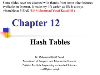
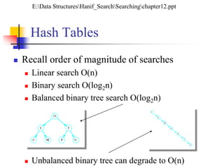
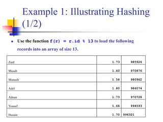
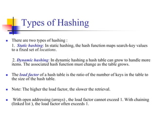
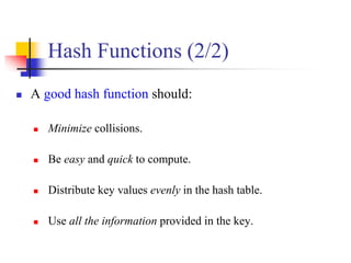
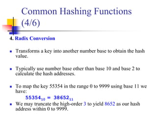
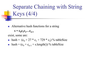
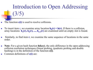
The most common probe sequences are of the form:
hi(key) = [h(key) + c(i)] % n, for i = 0, 1, …, n-1.
where h is a hash function and n is the size of the hash table
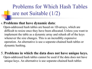
The function c(i) is required to have the following two properties:
Property 1:
c(0) = 0
Property 2:
The set of values {c(0) % n, c(1) % n, c(2) % n, . . . , c(n-1) % n} must be a
permutation of {0, 1, 2,. . ., n – 1}, that is, it must contain every integer between 0 and
n - 1 inclusive.
(2/5)

 The function c(i) is used to resolve collisions.
 To insert item r, we examine array location h0(r) = h(r). If there is a collision,
array locations h1(r), h2(r), ..., hn-1(r) are examined until an empty slot is found.
 Similarly, to find item r, we examine the same sequence of locations in the same
order.
 Note: For a given hash function h(key), the only difference in the open addressing
collision resolution techniques (linear probing, quadratic probing and double
hashing) is in the definition of the function c(i).
 Common definitions of c(i) are:
(3/5)

Collision resolution technique c(i)
Linear probing i
Quadratic probing ±i2
Double hashing i*hp(key)
where hp(key) is another hash function.
(4/5)

 Advantages of Open addressing:
 All items are stored in the hash table itself. There is no need
for another data structure.
 Open addressing is more efficient storage-wise.
 Disadvantages of Open Addressing:
 The keys of the objects to be hashed must be distinct.
 Dependent on choosing a proper table size.
 Requires the use of a three-state (Occupied, Empty, or
Deleted) flag in each cell.
(5/5)

Open Addressing Facts
 In general, primes give the best table sizes.
 With any open addressing method of collision resolution, as the
table fills, there can be a severe degradation in the table
performance.
 Load factors between 0.6 and 0.7 are common.
 Load factors > 0.7 are undesirable.
 The search time depends only on the load factor, not on the table
size.
 We can use the desired load factor to determine appropriate table
size:

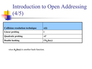
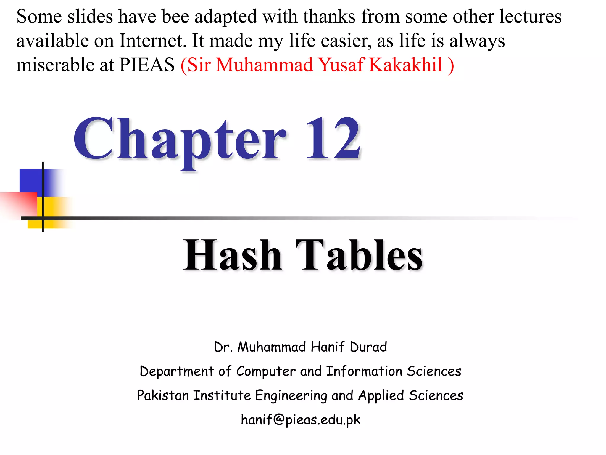
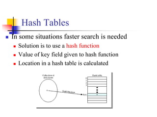
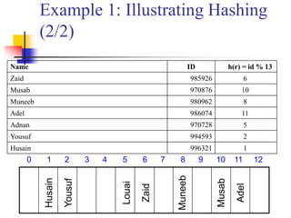
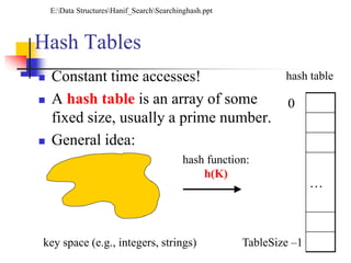
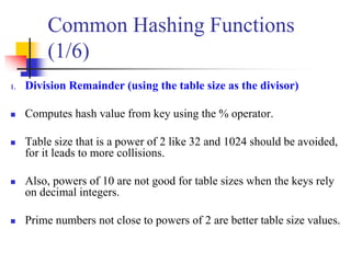
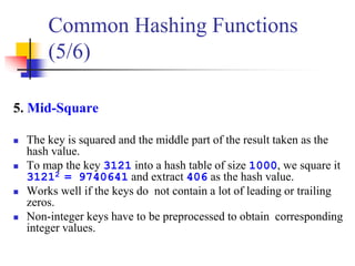
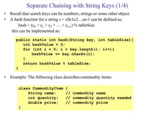
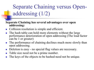
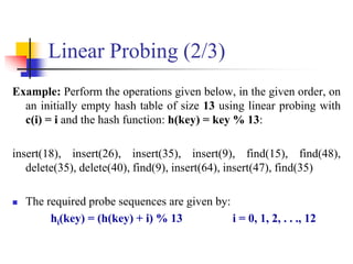
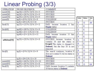
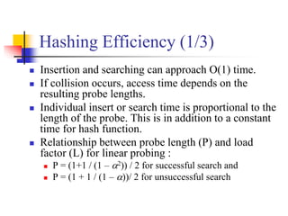
Linear Probing (1/3)
 c(i) is a linear function in i of the form c(i) = a*i.
 Usually c(i) is chosen as:
c(i) = i for i = 0, 1, . . . , tableSize – 1
 The probe sequences are then given by:
hi(key) = [h(key) + i] % tableSize for i = 0, 1, . . . , tableSize – 1
 For c(i) = a*i to satisfy Property 2, a and n must be relatively
prime.
Probe number key Auxiliary hash function

Example: Perform the operations given below, in the given order, on
an initially empty hash table of size 13 using linear probing with
c(i) = i and the hash function: h(key) = key % 13:
insert(18), insert(26), insert(35), insert(9), find(15), find(48),
delete(35), delete(40), find(9), insert(64), insert(47), find(35)
 The required probe sequences are given by:
hi(key) = (h(key) + i) % 13 i = 0, 1, 2, . . ., 12

Index Status Valu
e
0 O 26
1 E
2 E
3 E
4 E
5 O 18
6 E
7 E
8 O 47
9 D 35
10 O 9
11 E
12 O 64

Disadvantage of Linear Probing:
Primary Clustering (1/2)
 Linear probing is subject to a primary clustering phenomenon.
 Elements tend to cluster around table locations that they
originally hash to.
 Primary clusters can combine to form larger clusters. This leads
to long probe sequences and hence deterioration in hash table
efficiency.

Disadvantage of Linear Probing:
Primary Clustering (2/2)
Example of a primary cluster: Insert keys: 18, 41, 22, 44, 59, 32, 31, 73, in
this order, in an originally empty hash table of size 13, using the hash function
h(key) = key % 13 and c(i) = i:
h(18) = 5
h(41) = 2
h(22) = 9
h(44) = 5+1
h(59) = 7
h(32) = 6+1+1
h(31) = 5+1+1+1+1+1
h(73) = 8+1+1+1

Collision Resolution: Open
Addressing
 Quadratic Probing
 Double Hashing
 Rehashing
 Algorithms for:
 insert
 find
 withdraw

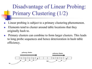
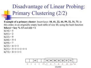
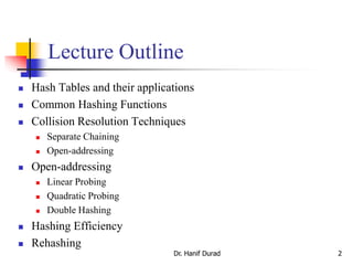
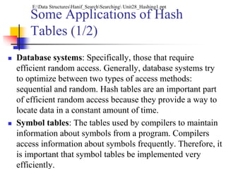
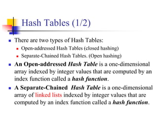
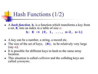
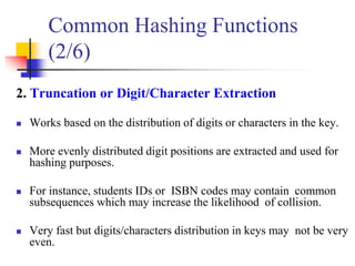
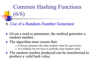
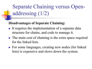
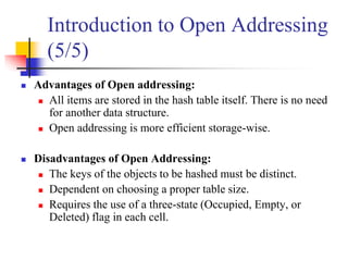
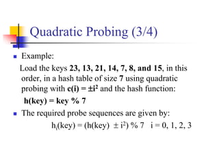
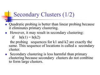
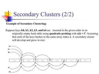
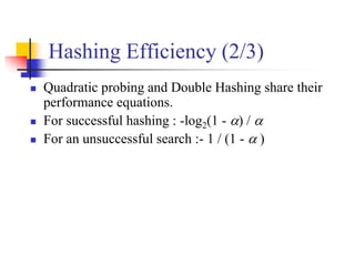
Quadratic Probing (1/4)
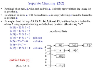
 Quadratic probing eliminates primary clusters.
 c(i) is a quadratic function in i of the form c(i) = a*i2 + b*i. Usually c(i) is
chosen as:
c(i) = i2 for i = 0, 1, . . . , tableSize – 1
or
c(i) = i2 for i = 0, 1, . . . , (tableSize – 1) / 2
 The probe sequences are then given by:
hi(key) = [h(key) + i2] % tableSize for i = 0, 1, . . . , tableSize – 1
or
hi(key) = [h(key)  i2] % tableSize for i = 0, 1, . . . , (tableSize – 1) / 2
Probe number key Auxiliary hash function

Note for Quadratic Probing (2/4)
 Hashtable size should not be an even number;
otherwise Property 2 will not be satisfied.
 Ideally, table size should be a prime of the form 4j+3,
where j is an integer. This choice of table size
guarantees Property 2.

 Example:
Load the keys 23, 13, 21, 14, 7, 8, and 15, in this
order, in a hash table of size 7 using quadratic
probing with c(i) = i2 and the hash function:
h(key) = key % 7
 The required probe sequences are given by:
hi(key) = (h(key)  i2) % 7 i = 0, 1, 2, 3

h0(23) = (23 % 7) % 7 = 2
h0(13) = (13 % 7) % 7 = 6
h0(21) = (21 % 7) % 7 = 0
h0(14) = (14 % 7) % 7 = 0 collision
h1(14) = (0 + 12) % 7 = 1
h0(7) = (7 % 7) % 7 = 0 collision
h1(7) = (0 + 12) % 7 = 1 collision
h-1(7) = (0 - 12) % 7 = -1
NORMALIZE: (-1 + 7) % 7 = 6 collision
h2(7) = (0 + 22) % 7 = 4
h0(8) = (8 % 7)%7 = 1 collision
h1(8) = (1 + 12) % 7 = 2 collision
h-1(8) = (1 - 12) % 7 = 0 collision
h2(8) = (1 + 22) % 7 = 5
h0(15) = (15 % 7)%7 = 1 collision
h1(15) = (1 + 12) % 7 = 2 collision
h-1(15) = (1 - 12) % 7 = 0 collision
h2(15) = (1 + 22) % 7 = 5 collision
h-2(15) = (1 - 22) % 7 = -3
NORMALIZE: (-3 + 7) % 7 = 4 collision
h3(15) = (1 + 32)%7 = 3
hi(key) = (h(key)  i2) % 7 i = 0, 1, 2, 3
0 O 21
1 O 14
2 O 23
3 O 15
4 O 7
5 O 8
6 O 13

Secondary Clusters (1/2)
 Quadratic probing is better than linear probing because
it eliminates primary clustering.
 However, it may result in secondary clustering:
if h(k1) = h(k2)
the probing sequences for k1 and k2 are exactly the
same. This sequence of locations is called a secondary
cluster.
 Secondary clustering is less harmful than primary
clustering because secondary clusters do not combine
to form large clusters.

Secondary Clusters (2/2)
Example of Secondary Clustering:
Suppose keys k0, k1, k2, k3, and k4 are inserted in the given order in an
originally empty hash table using quadratic probing with c(i) = i2. Assuming
that each of the keys hashes to the same array index x. A secondary cluster
will develop and grow in size:

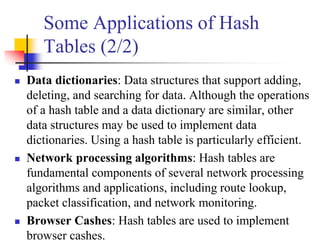
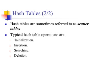
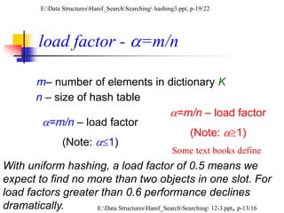
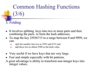
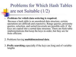
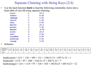
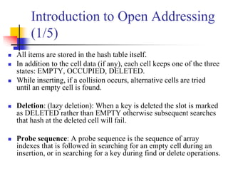
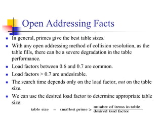
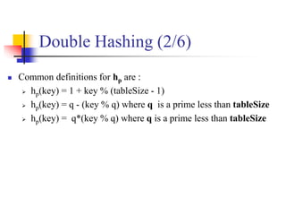
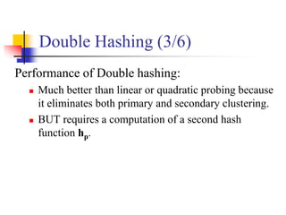
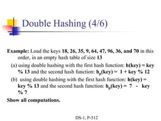
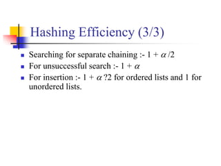
Double Hashing (1/6)
 To eliminate secondary clustering, synonyms must have different probe sequences.
 Double hashing achieves this by having two hash functions that both depend on the
hash key.
c(i) = i * hp(key) for i = 0, 1, . . . , tableSize – 1
where hp (or h2) is another hash function.
 The probing sequence is:
hi(key) = [h(key) + i*hp(key)]% tableSize for i = 0, 1, . . . , tableSize – 1
 The function c(i) = i*hp(r) satisfies Property 2 provided hp(r) and tableSize are
relatively prime.
DS-1, P-512

 Common definitions for hp are :
 hp(key) = 1 + key % (tableSize - 1)
 hp(key) = q - (key % q) where q is a prime less than tableSize
 hp(key) = q*(key % q) where q is a prime less than tableSize

Performance of Double hashing:
 Much better than linear or quadratic probing because
it eliminates both primary and secondary clustering.
 BUT requires a computation of a second hash
function hp.

Example: Load the keys 18, 26, 35, 9, 64, 47, 96, 36, and 70 in this
order, in an empty hash table of size 13
(a) using double hashing with the first hash function: h(key) = key
% 13 and the second hash function: hp(key) = 1 + key % 12
(b) using double hashing with the first hash function: h(key) =
key % 13 and the second hash function: hp(key) = 7 - key
% 7
Show all computations.
DS-1, P-512

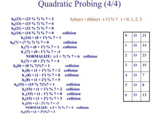
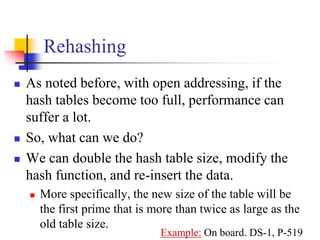
h0(18) = (18%13)%13 = 5
h0(26) = (26%13)%13 = 0
h0(35) = (35%13)%13 = 9
h0(9) = (9%13)%13 = 9 collision
hp(9) = 1 + 9%12 = 10
h1(9) = (9 + 1*10)%13 = 6
h0(64) = (64%13)%13 = 12
h0(47) = (47%13)%13 = 8
h0(96) = (96%13)%13 = 5 collision
hp(96) = 1 + 96%12 = 1
h1(96) = (5 + 1*1)%13 = 6 collision
h2(96) = (5 + 2*1)%13 = 7
h0(36) = (36%13)%13 = 10
h0(70) = (70%13)%13 = 5 collision
hp(70) = 1 + 70%12 = 11
h1(70) = (5 + 1*11)%13 = 3
hi(key) = [h(key) + i*hp(key)]% 13
h(key) = key % 13
hp(key) = 1 + key % 12
DS-1, P-513

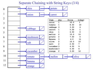
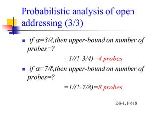
h0(18) = (18%13)%13 = 5
h0(26) = (26%13)%13 = 0
h0(35) = (35%13)%13 = 9
h0(9) = (9%13)%13 = 9 collision
hp(9) = 7 - 9%7 = 5
h1(9) = (9 + 1*5)%13 = 1
h0(64) = (64%13)%13 = 12
h0(47) = (47%13)%13 = 8
h0(96) = (96%13)%13 = 5 collision
hp(96) = 7 - 96%7 = 2
h1(96) = (5 + 1*2)%13 = 7
h0(36) = (36%13)%13 = 10
h0(70) = (70%13)%13 = 5 collision
hp(70) = 7 - 70%7 = 7
h1(70) = (5 + 1*7)%13 = 12 collision
h2(70) = (5 + 2*7)%13 = 6
hi(key) = [h(key) + i*hp(key)]% 13
h(key) = key % 13
hp(key) = 7 - key % 7

Probabilistic analysis of open
addressing (1/3)
n – number of elements in dictionary D
m – size of hash table
Assume that for every k,
h(k,0),…,h(k,m-1) is random permutation
=n/m – load factor (Note: 1)
Expected time of Insert or Find is:
E:Data StructuresHanif_SearchSearching hashing3.ppt, p-13/16

addressing (2/3)
Expected time of Insert or Find is:
Non rigorous proof:
If we choose a random element in the
table, the probability that it is full is .
The probability that the first i locations in the
probe sequence are all occupied is therefore i.

addressing (3/3)
 if =3/4,then upper-bound on number of
probes=?
=1/(1-3/4)=4 probes
 if =7/8,then upper-bound on number of
probes=?
=1/(1-7/8)=8 probes
DS-1, P-518

Hashing Efficiency (1/3)
 Insertion and searching can approach O(1) time.
 If collision occurs, access time depends on the
resulting probe lengths.
 Individual insert or search time is proportional to the
length of the probe. This is in addition to a constant
time for hash function.
 Relationship between probe length (P) and load
factor (L) for linear probing :
 P = (1+1 / (1 – 2)) / 2 for successful search and
 P = (1 + 1 / (1 – ))/ 2 for unsuccessful search

 Quadratic probing and Double Hashing share their
performance equations.
 For successful hashing : -log2(1 - ) / 
 For an unsuccessful search :- 1 / (1 -  )

 Searching for separate chaining :- 1 +  /2
 For unsuccessful search :- 1 + 
 For insertion :- 1 +  ?2 for ordered lists and 1 for
unordered lists.

Rehashing
 As noted before, with open addressing, if the
hash tables become too full, performance can
suffer a lot.
 So, what can we do?
 We can double the hash table size, modify the
hash function, and re-insert the data.
 More specifically, the new size of the table will be
the first prime that is more than twice as large as the
old table size.
Example: On board. DS-1, P-519

Chapter 12 ds

Recommended

Recommended

More Related Content

What's hot

What's hot (20)

Similar to Chapter 12 ds

Similar to Chapter 12 ds (20)

More from Hanif Durad

More from Hanif Durad (20)

Recently uploaded

Recently uploaded (20)

Chapter 12 ds