Download as PDF, PPTX
![Representation of Graphs
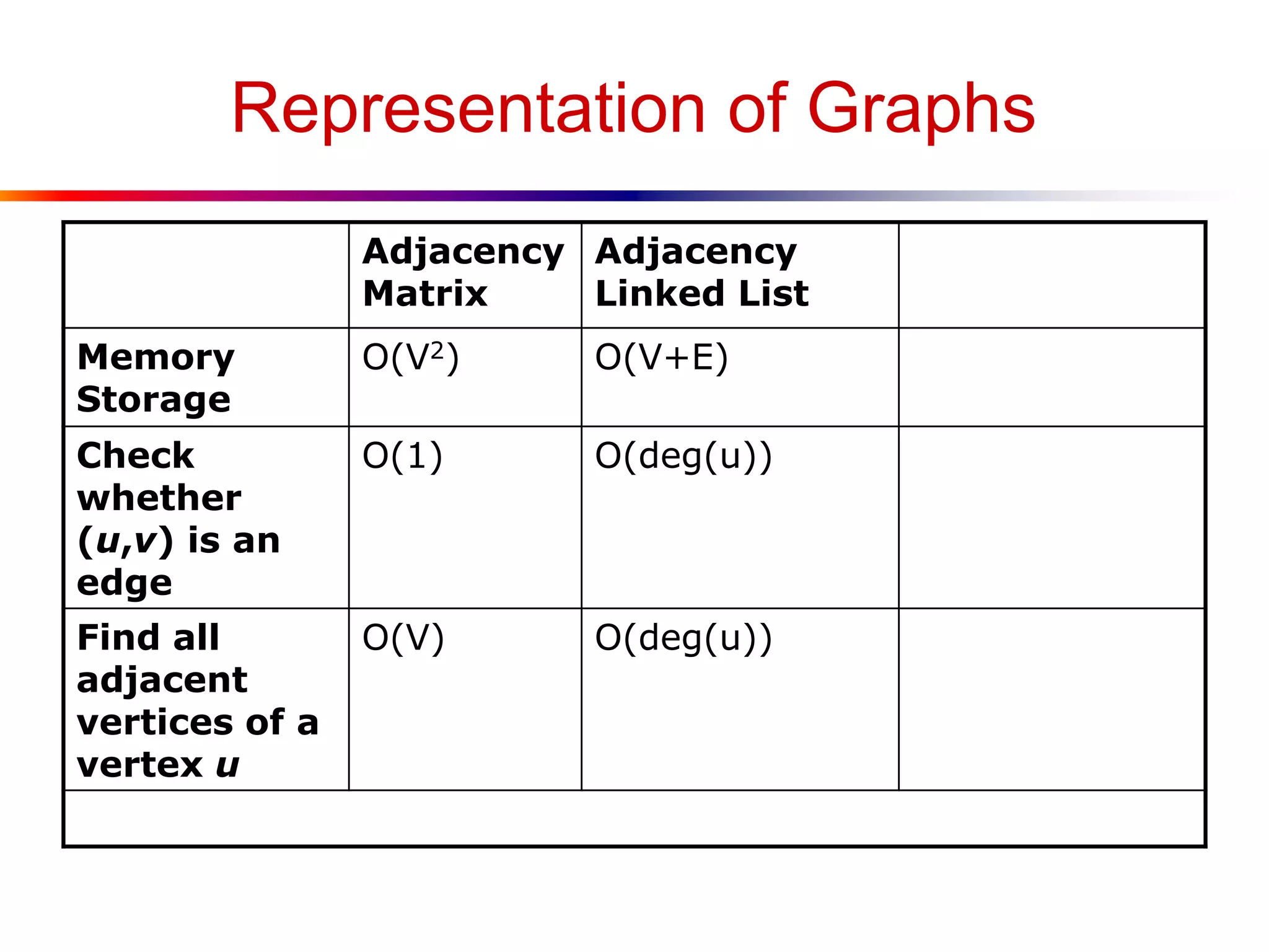
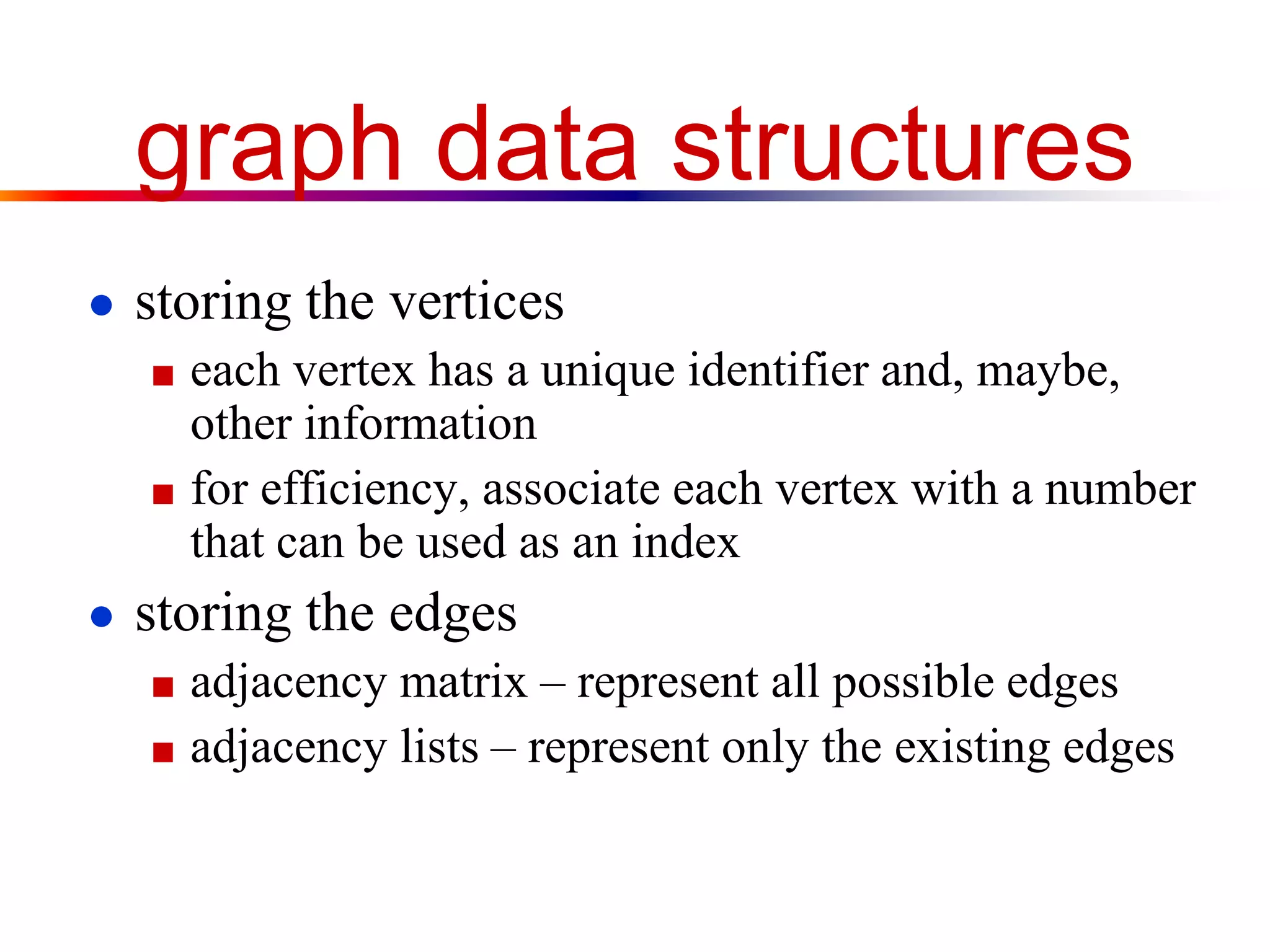
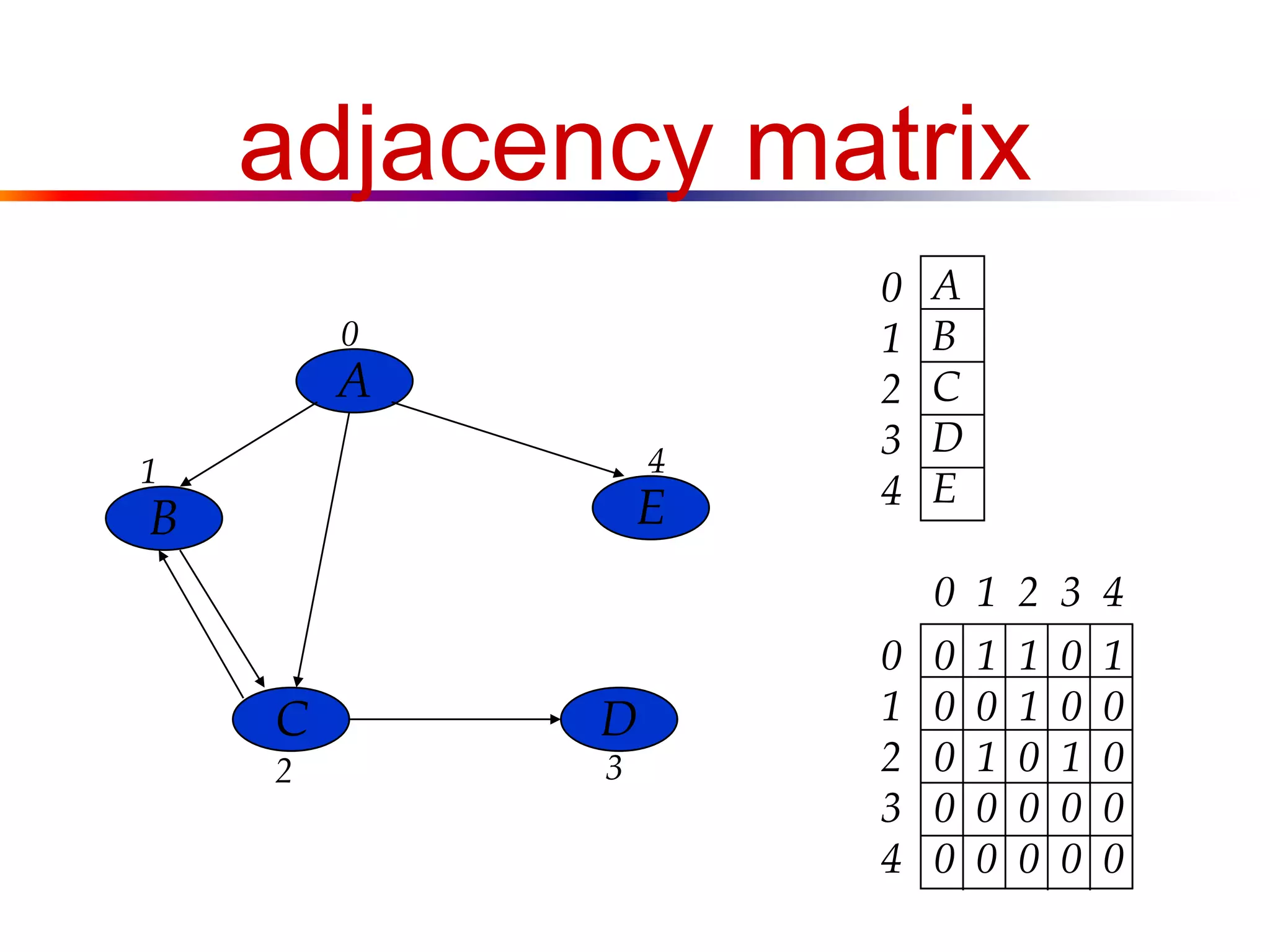
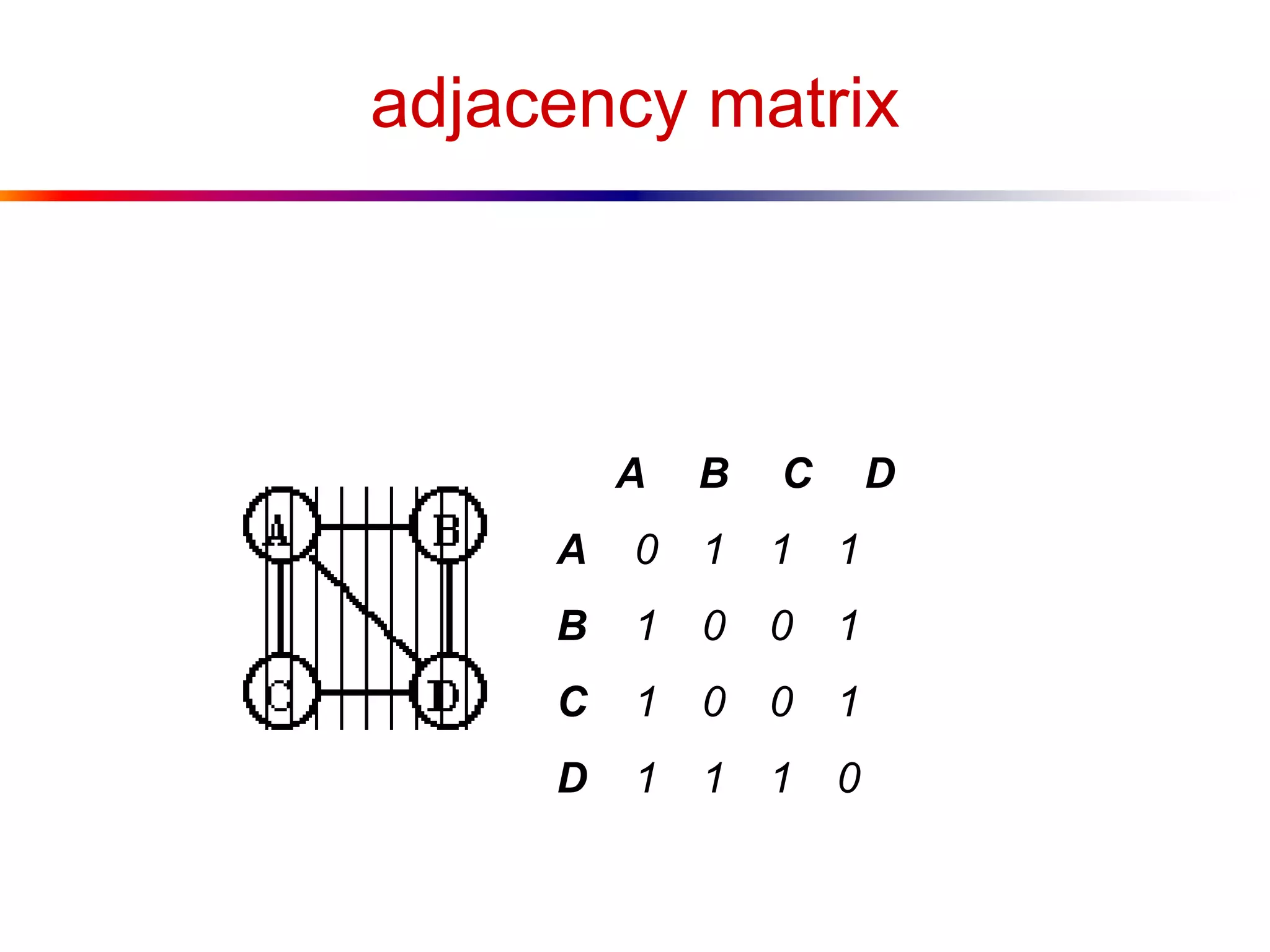
● Adjacency Matrix
■ A V x V array, with matrix[i][j] storing whether
there is an edge between the ith vertex and the jth
vertex
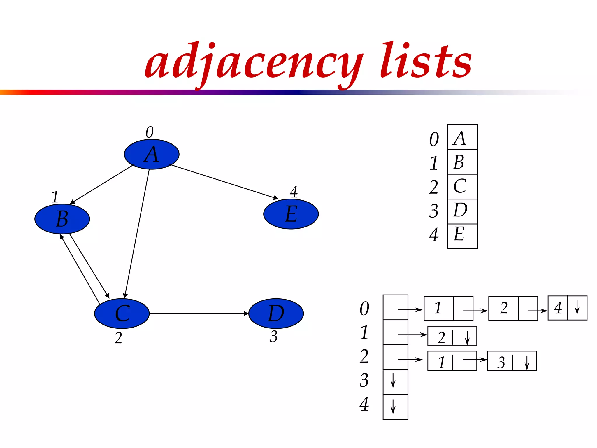
● Adjacency Linked List
■ One linked list per vertex, each storing directly
reachable vertices](https://image.slidesharecdn.com/lecture15-140420071734-phpapp01/75/Graph-13-2048.jpg)
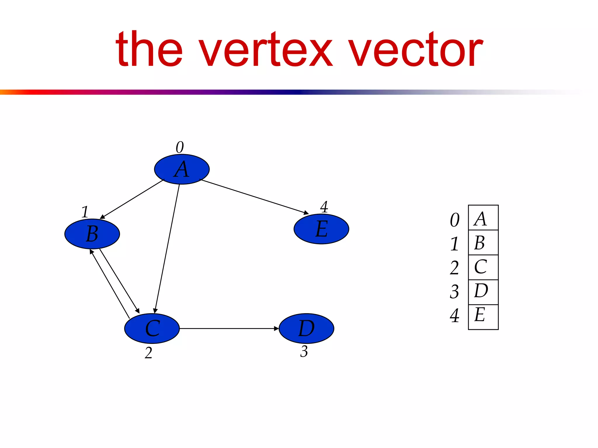
![a digraph
A
B
C D
E
V = [A, B, C, D, E]
E = [<A,B>, <B,C>, <C,B>, <A,C>, <A,E>, <C,D>]](https://image.slidesharecdn.com/lecture15-140420071734-phpapp01/75/Graph-16-2048.jpg)
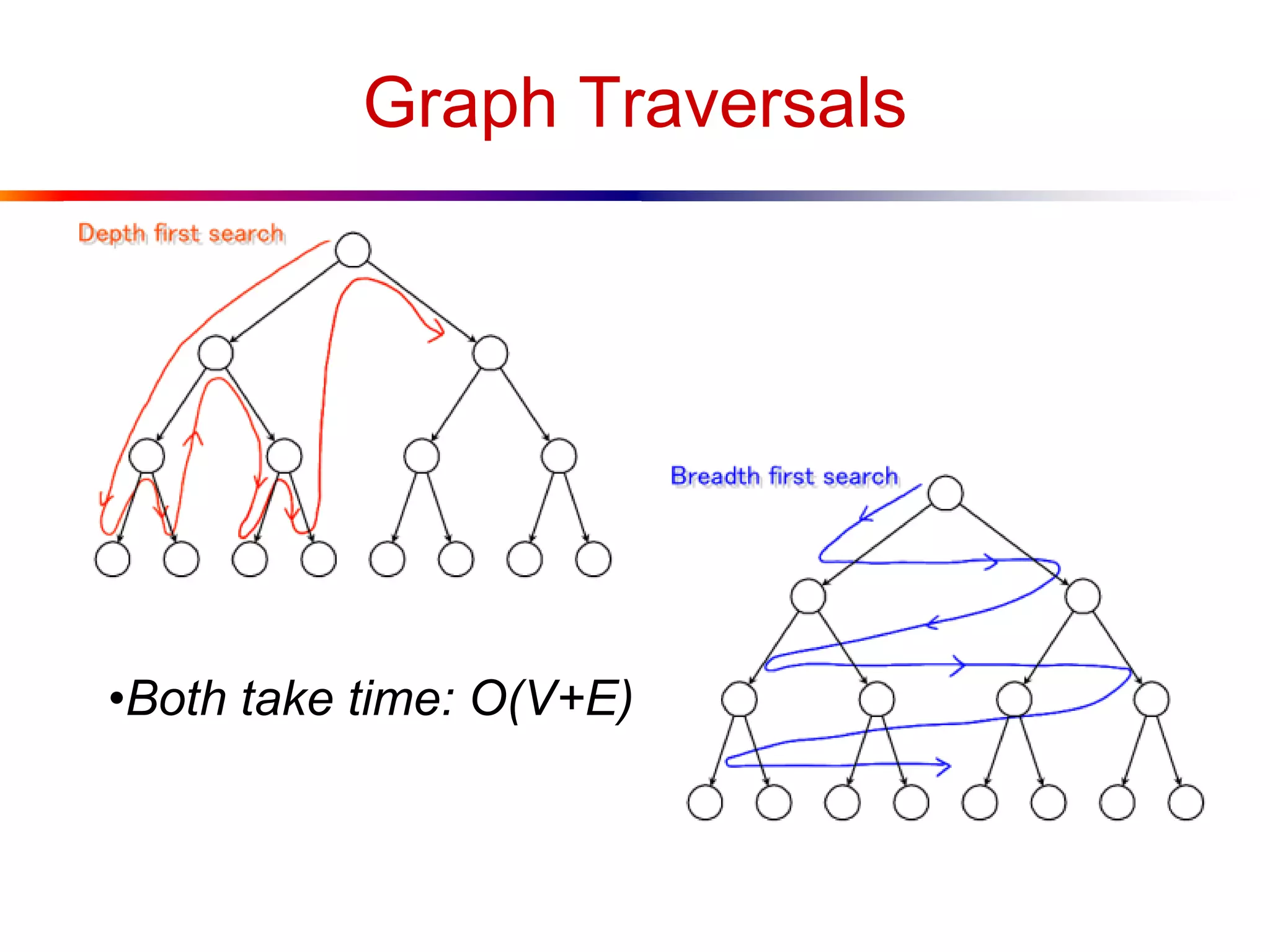
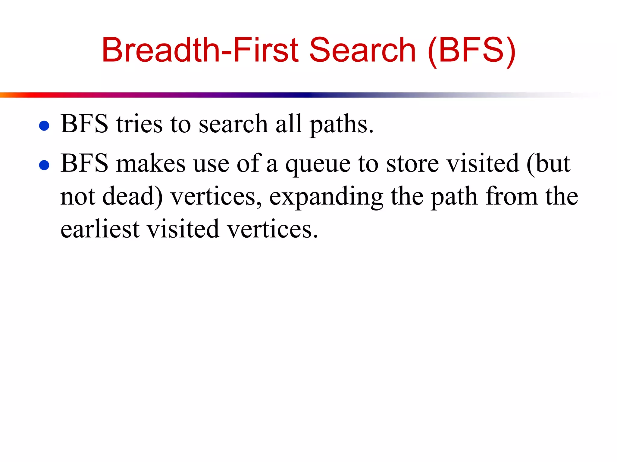
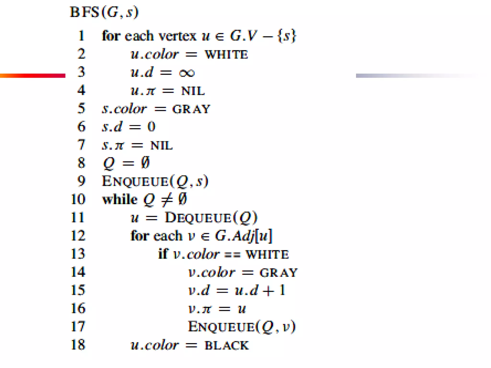
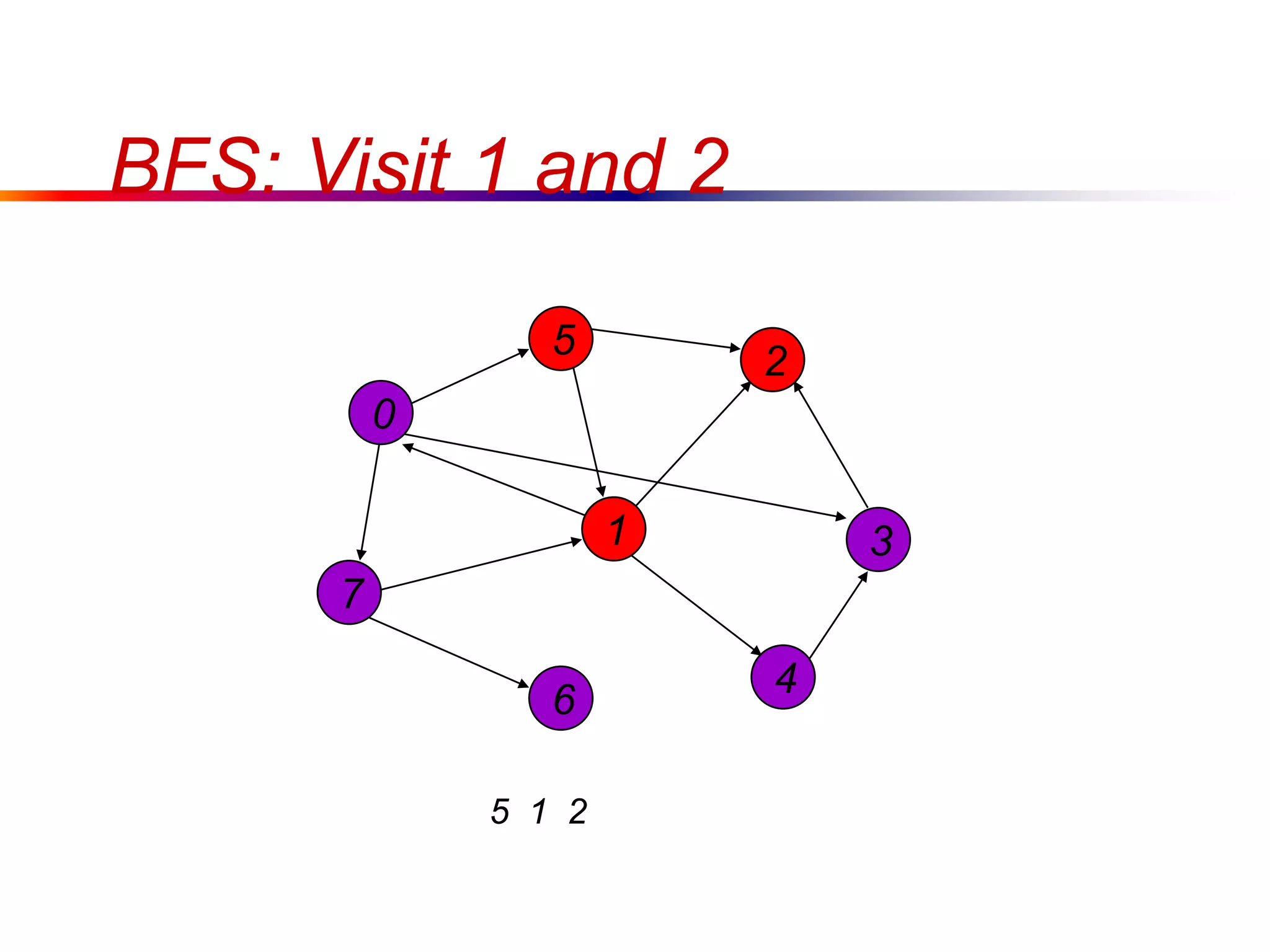
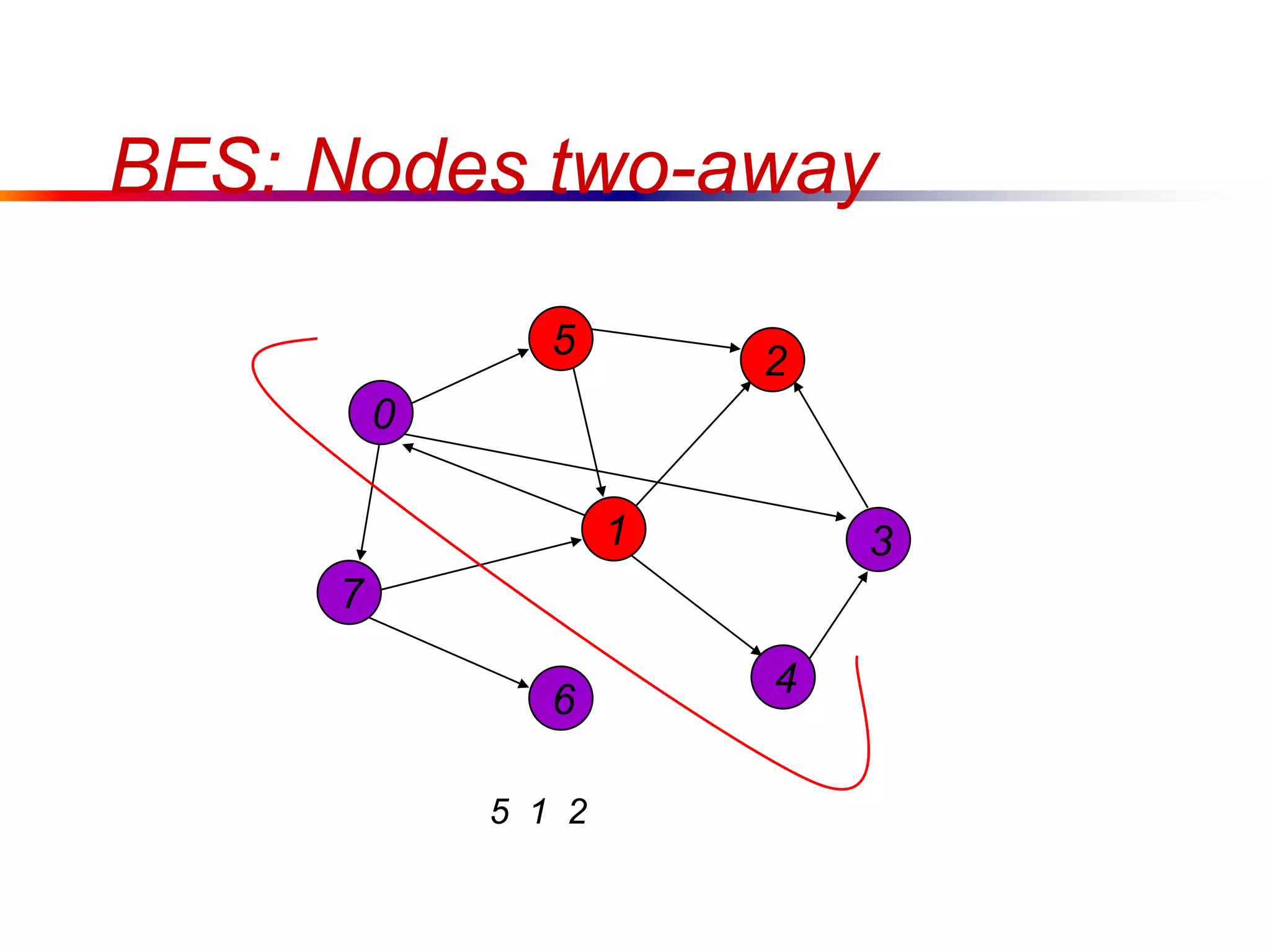
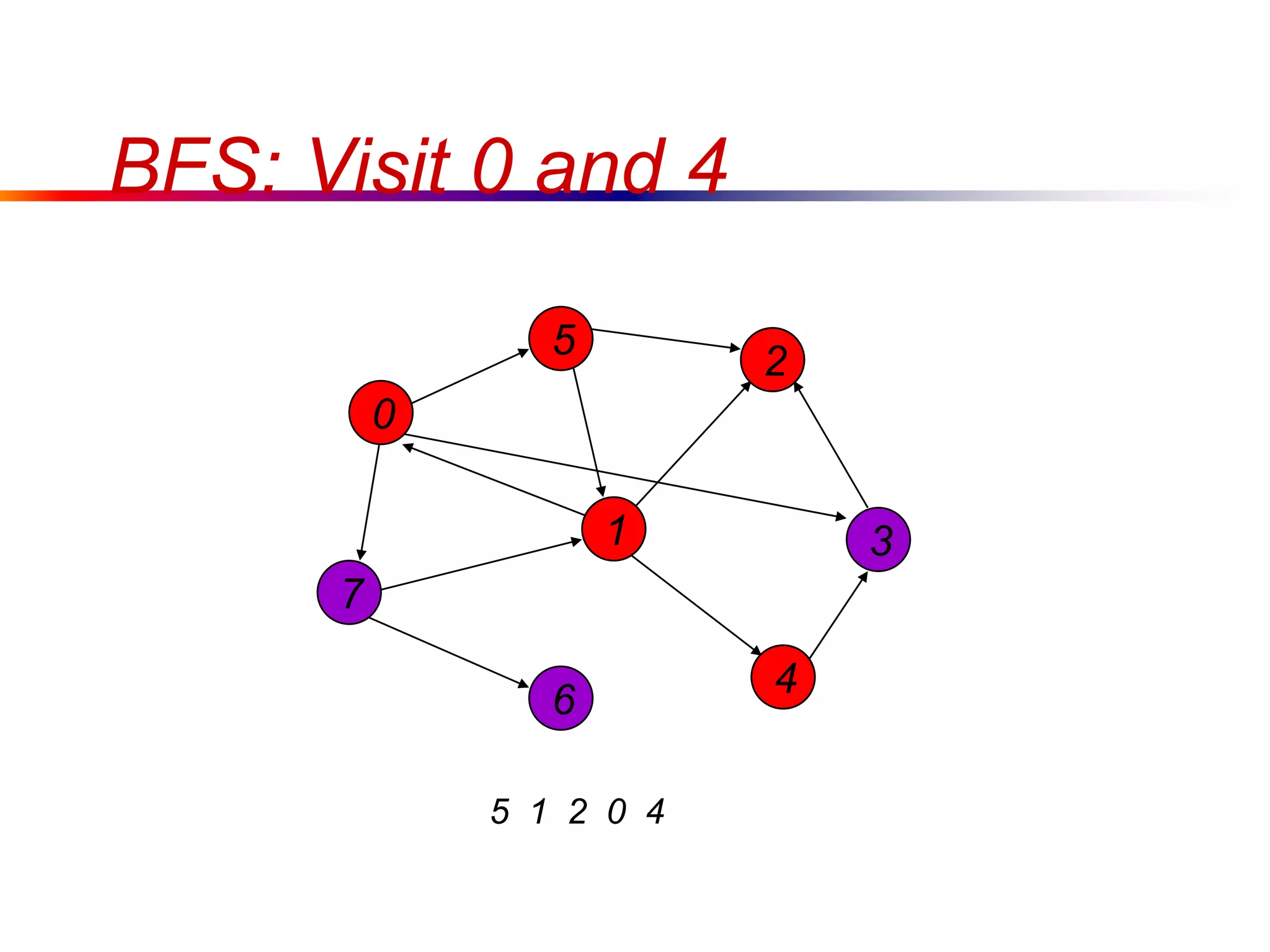
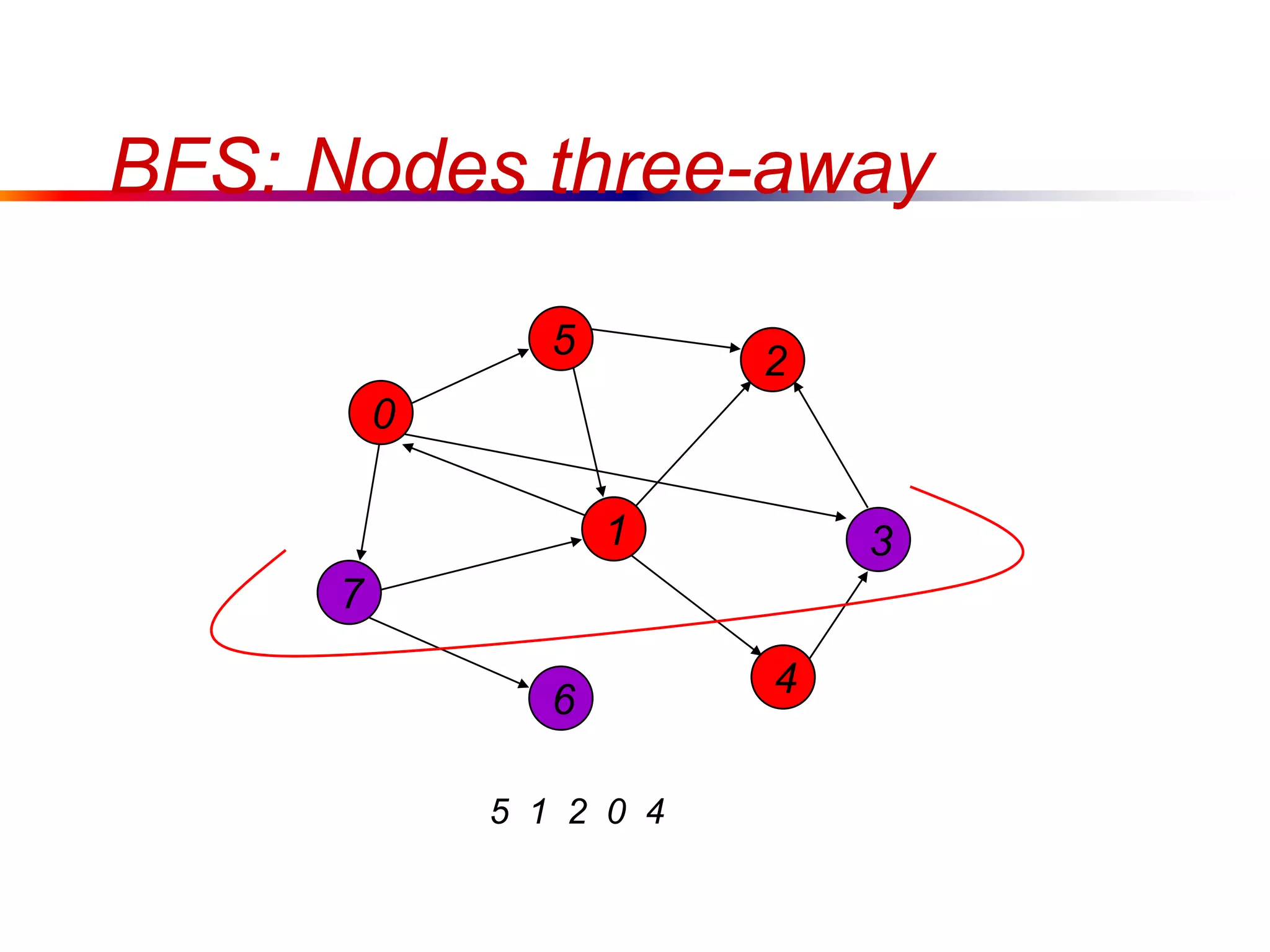
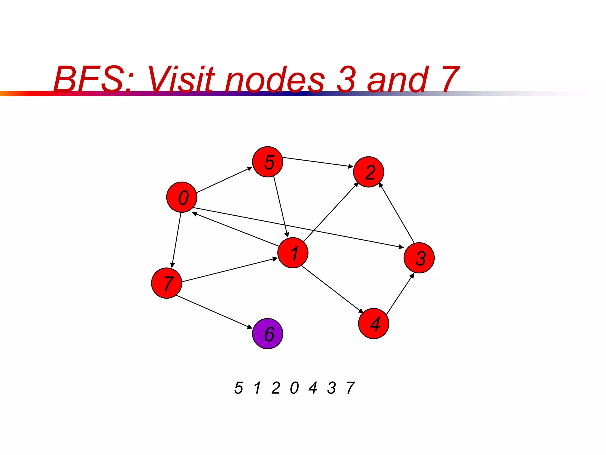

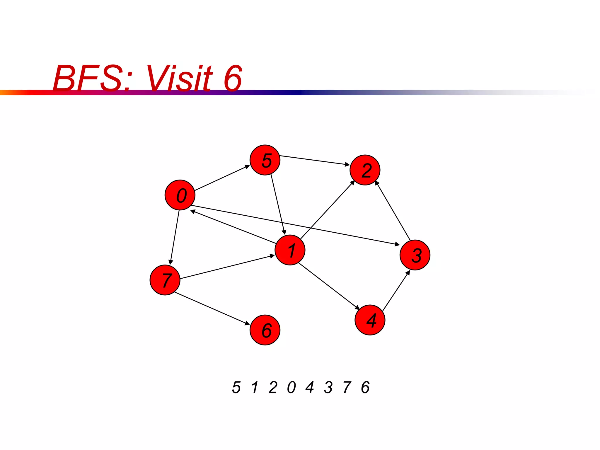
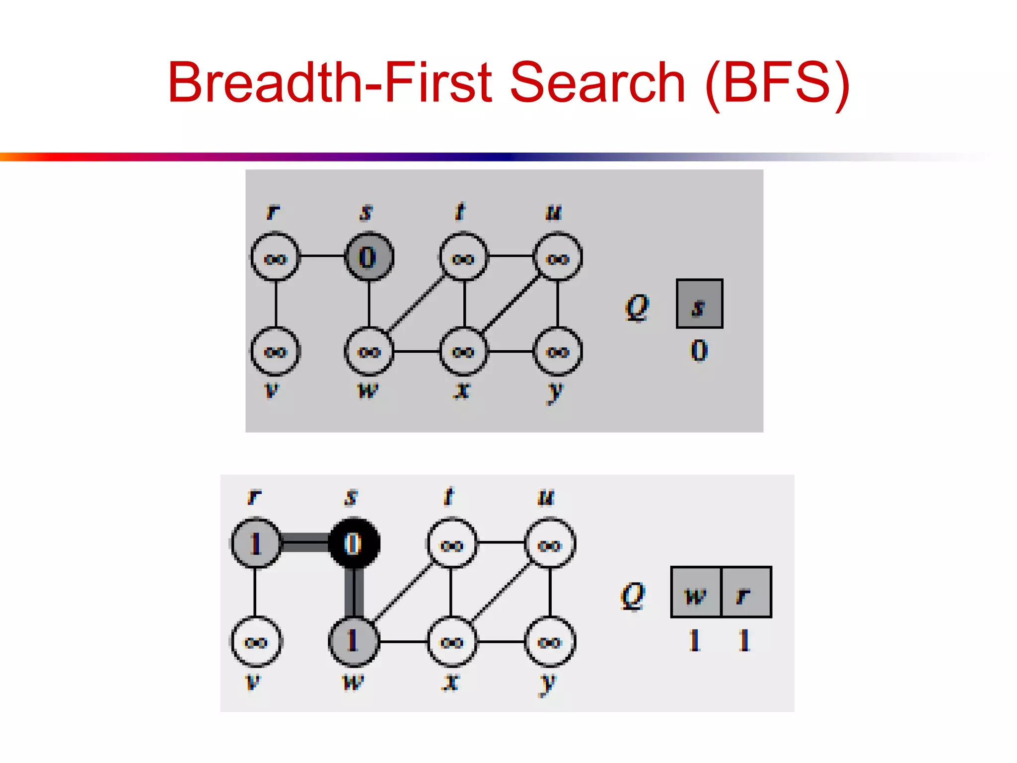
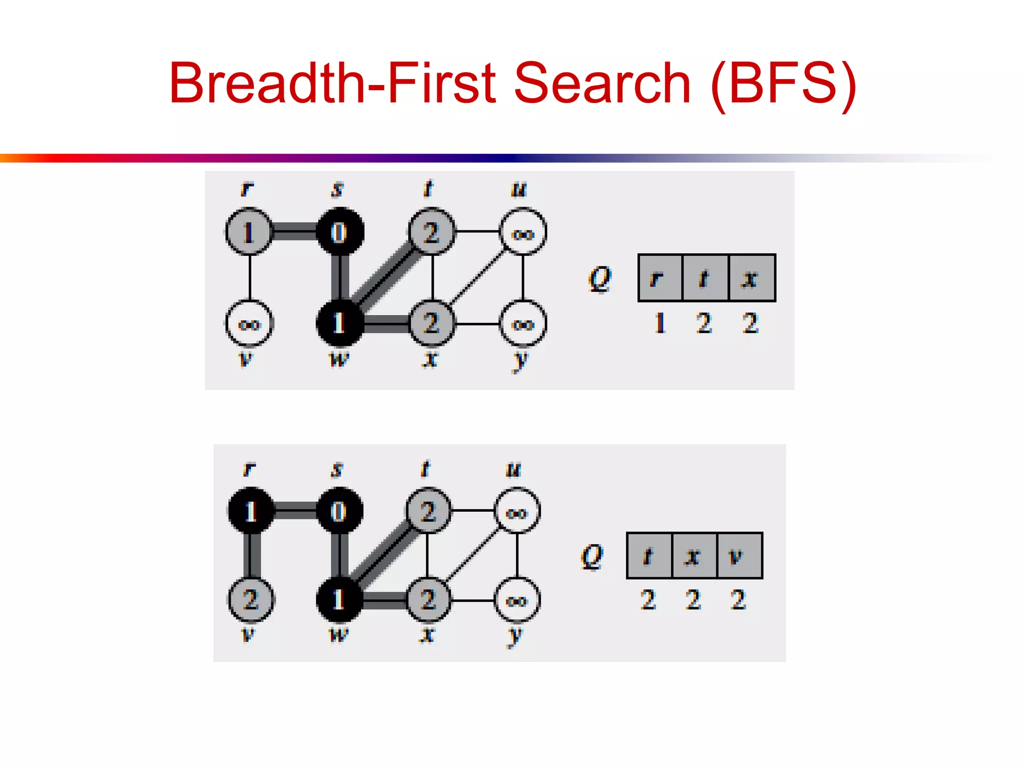

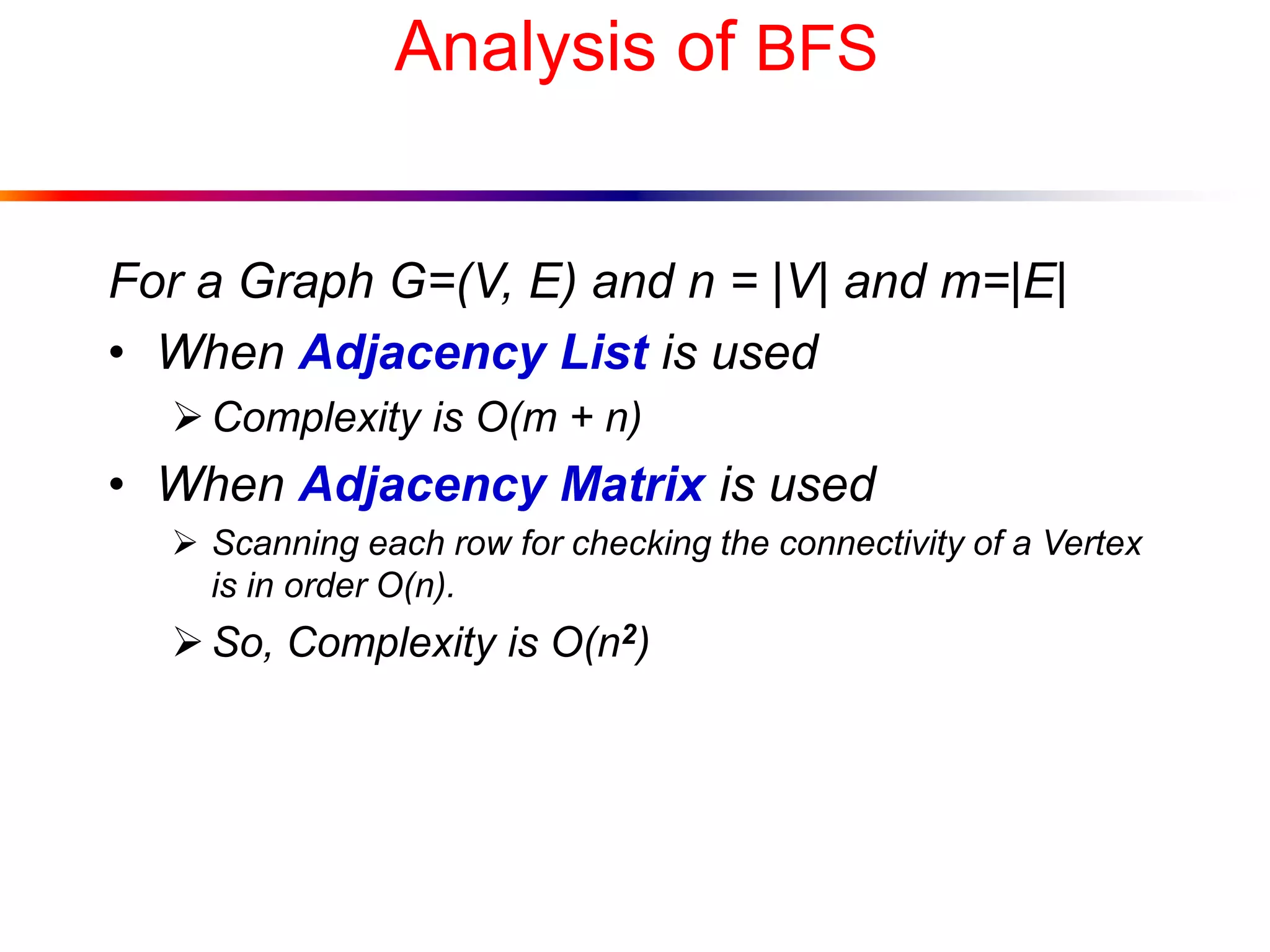
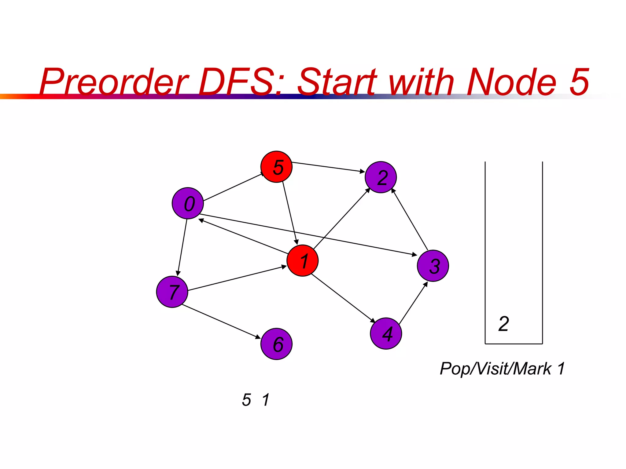
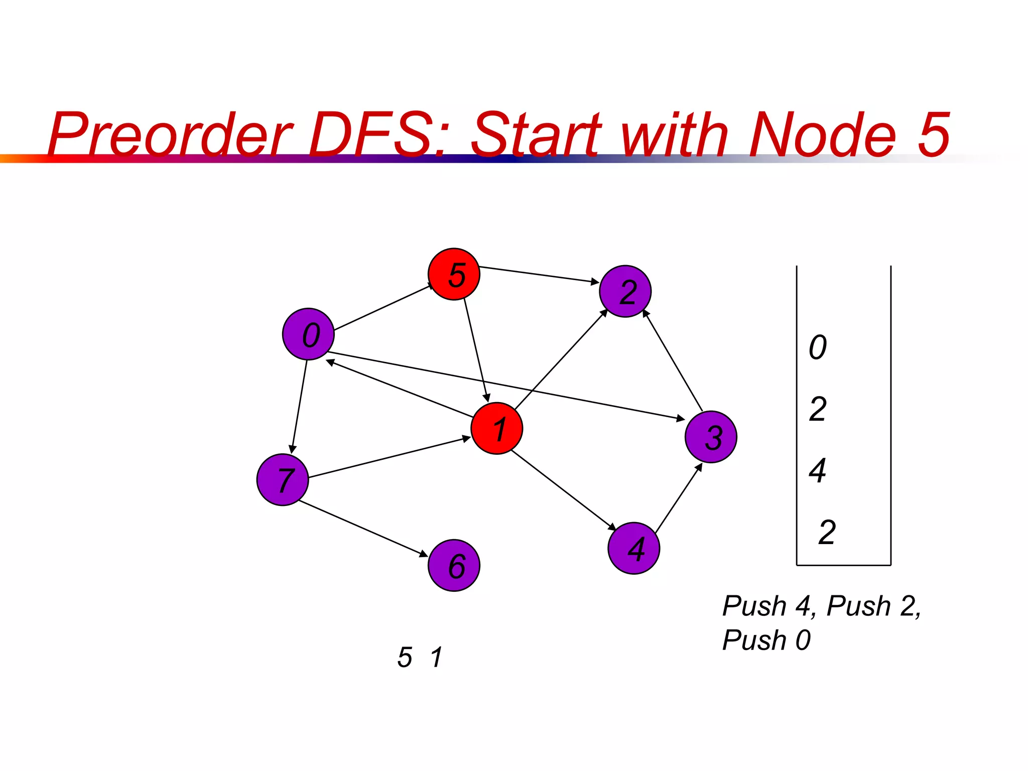
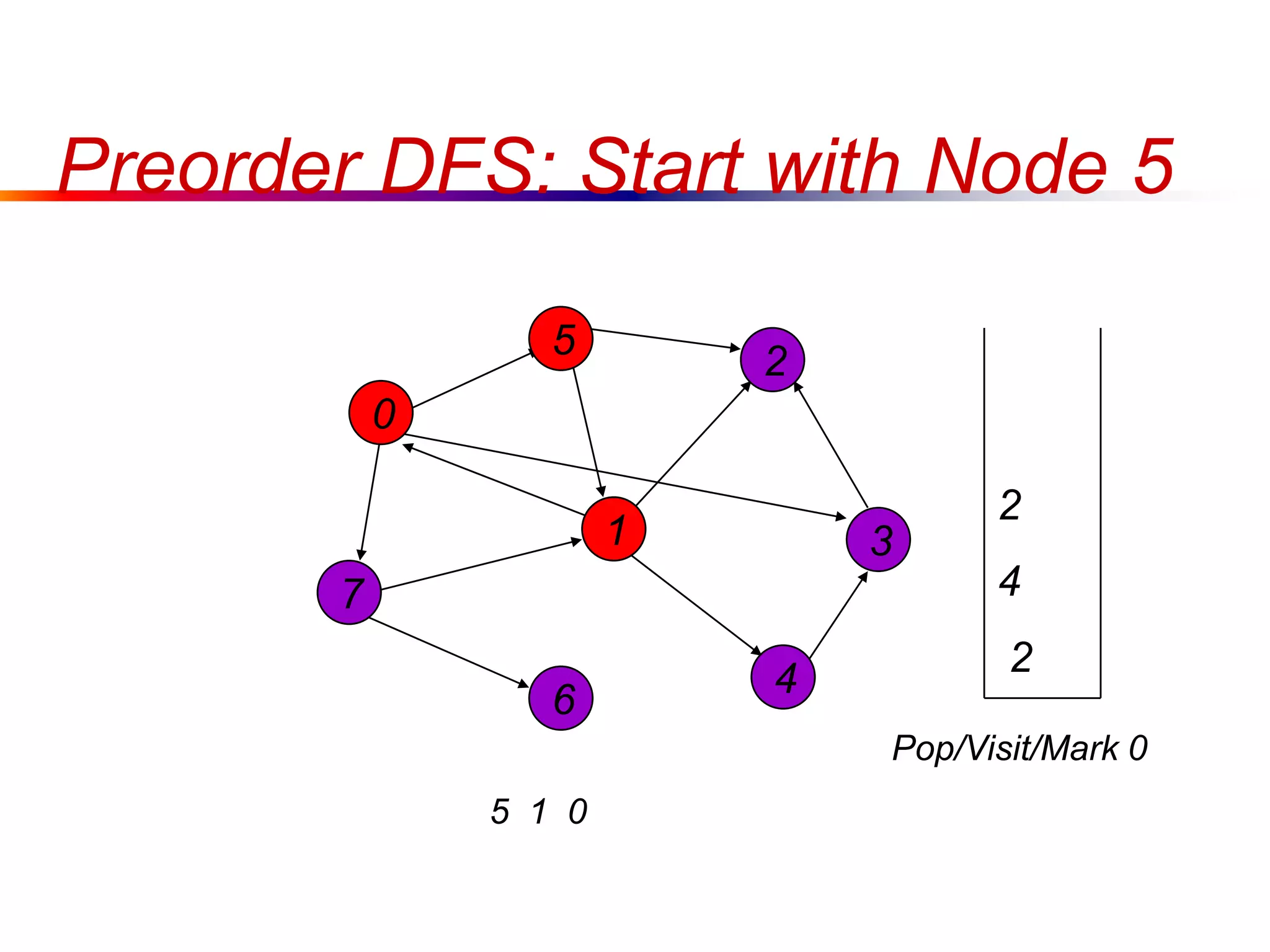
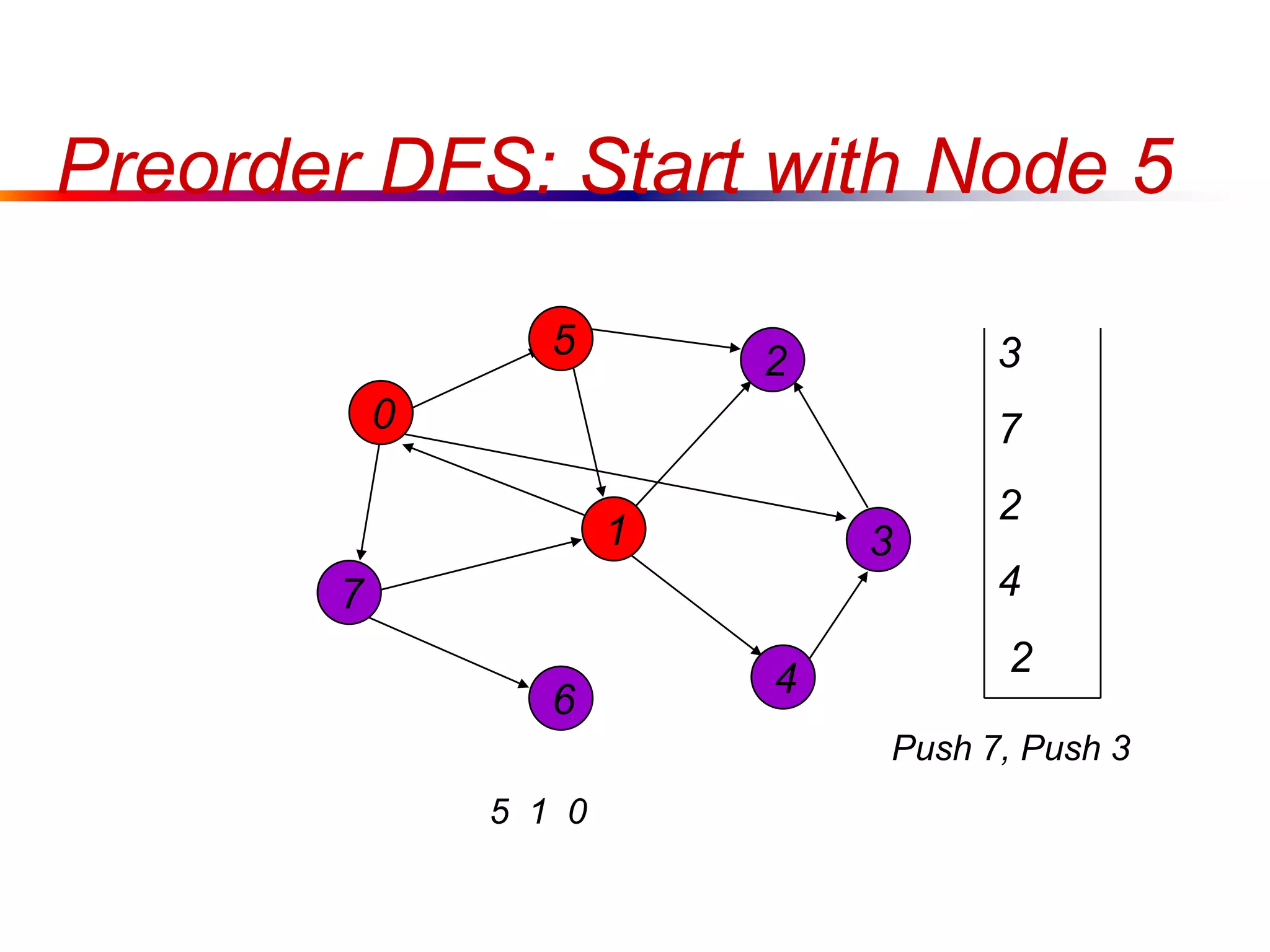
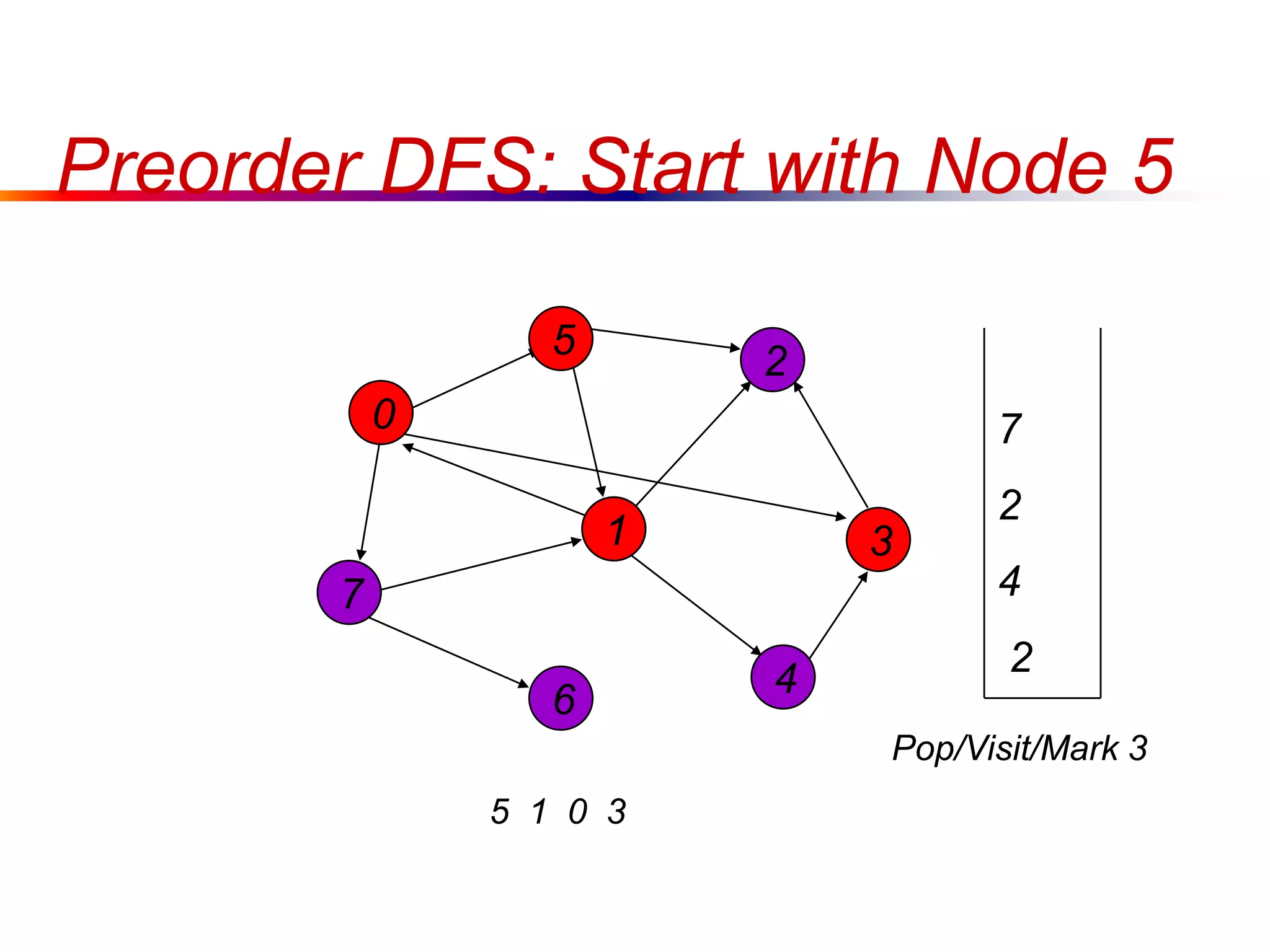
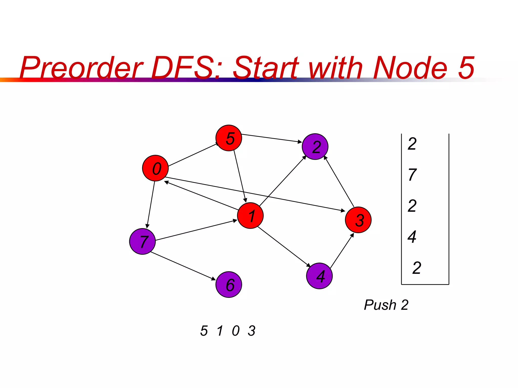
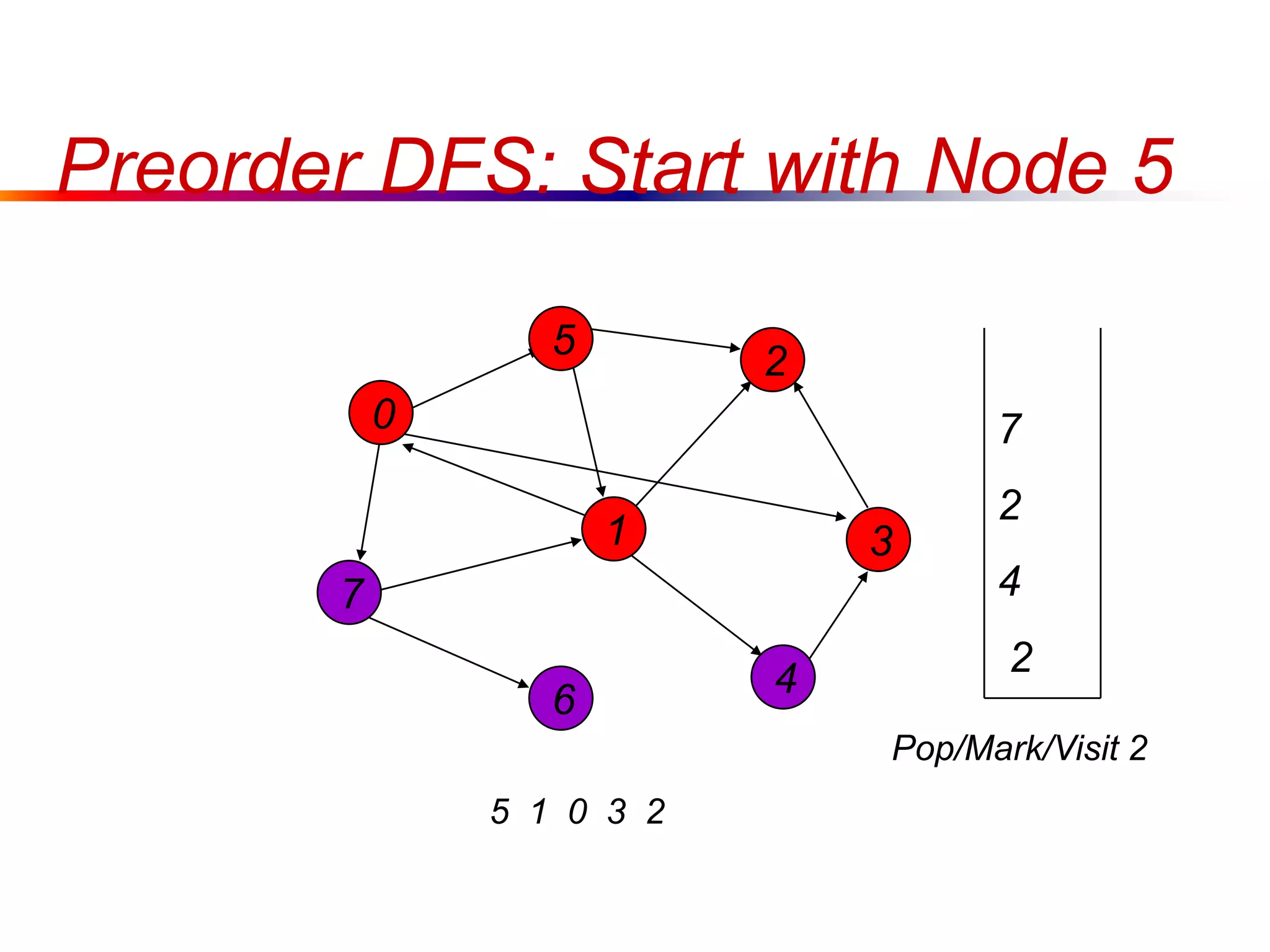
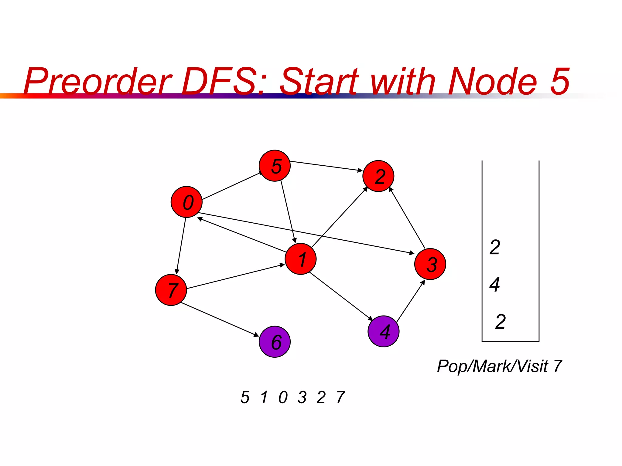
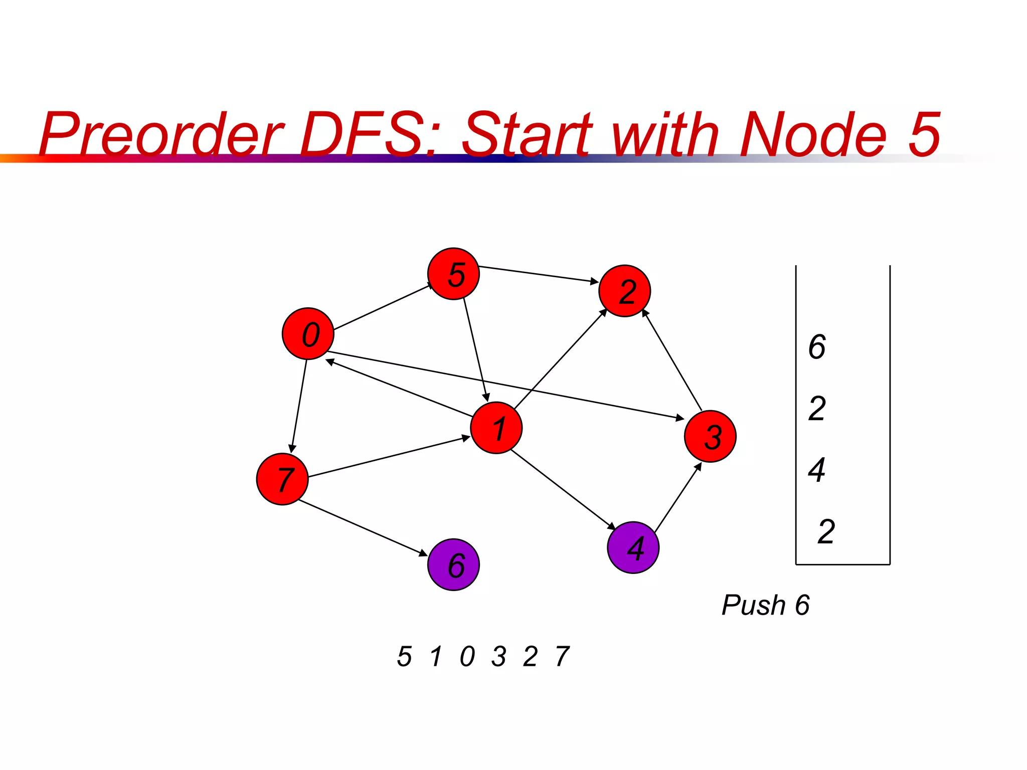
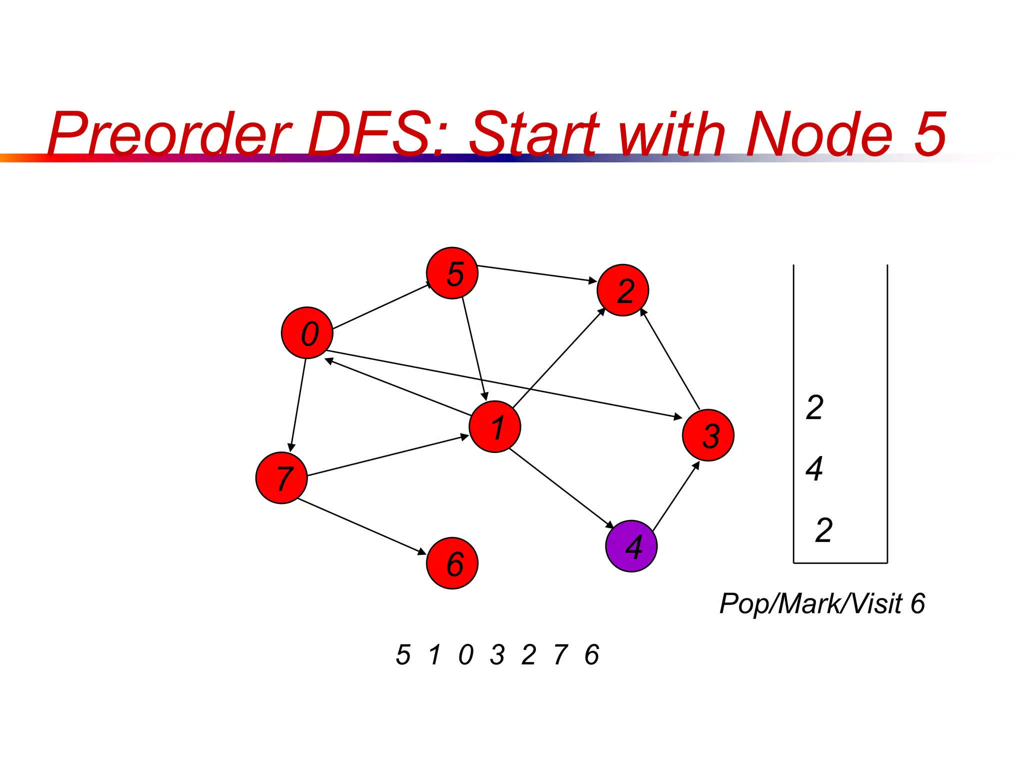
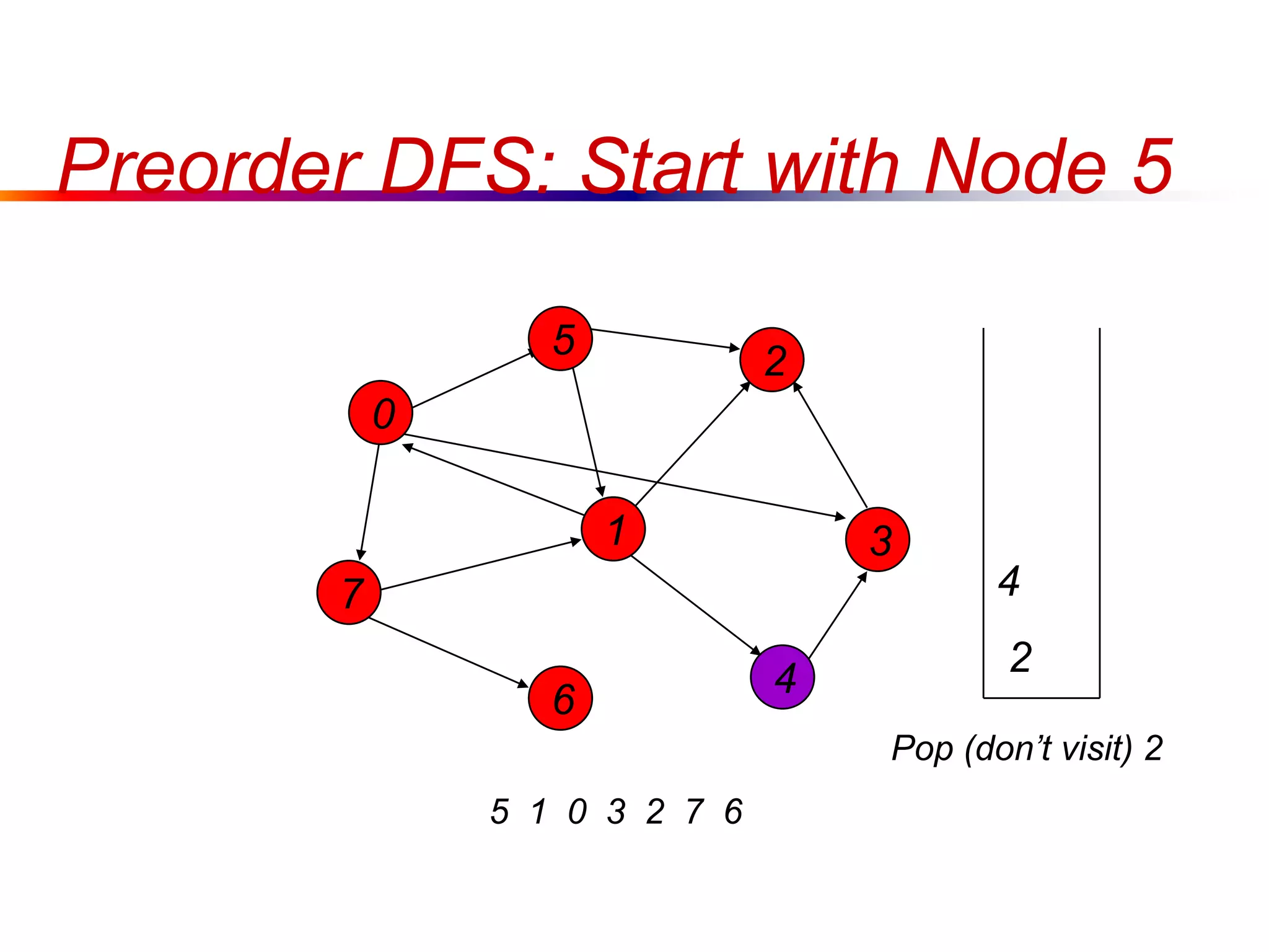
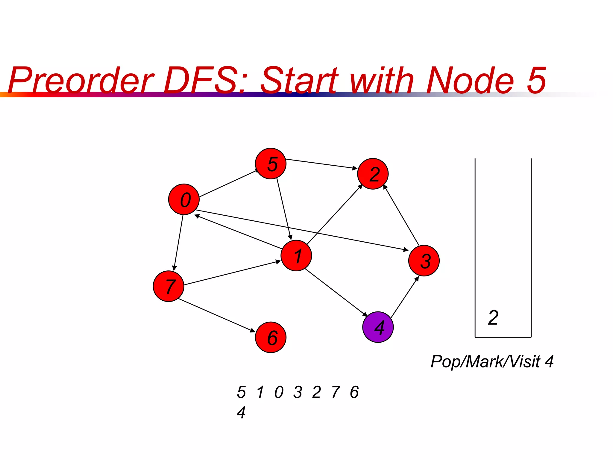
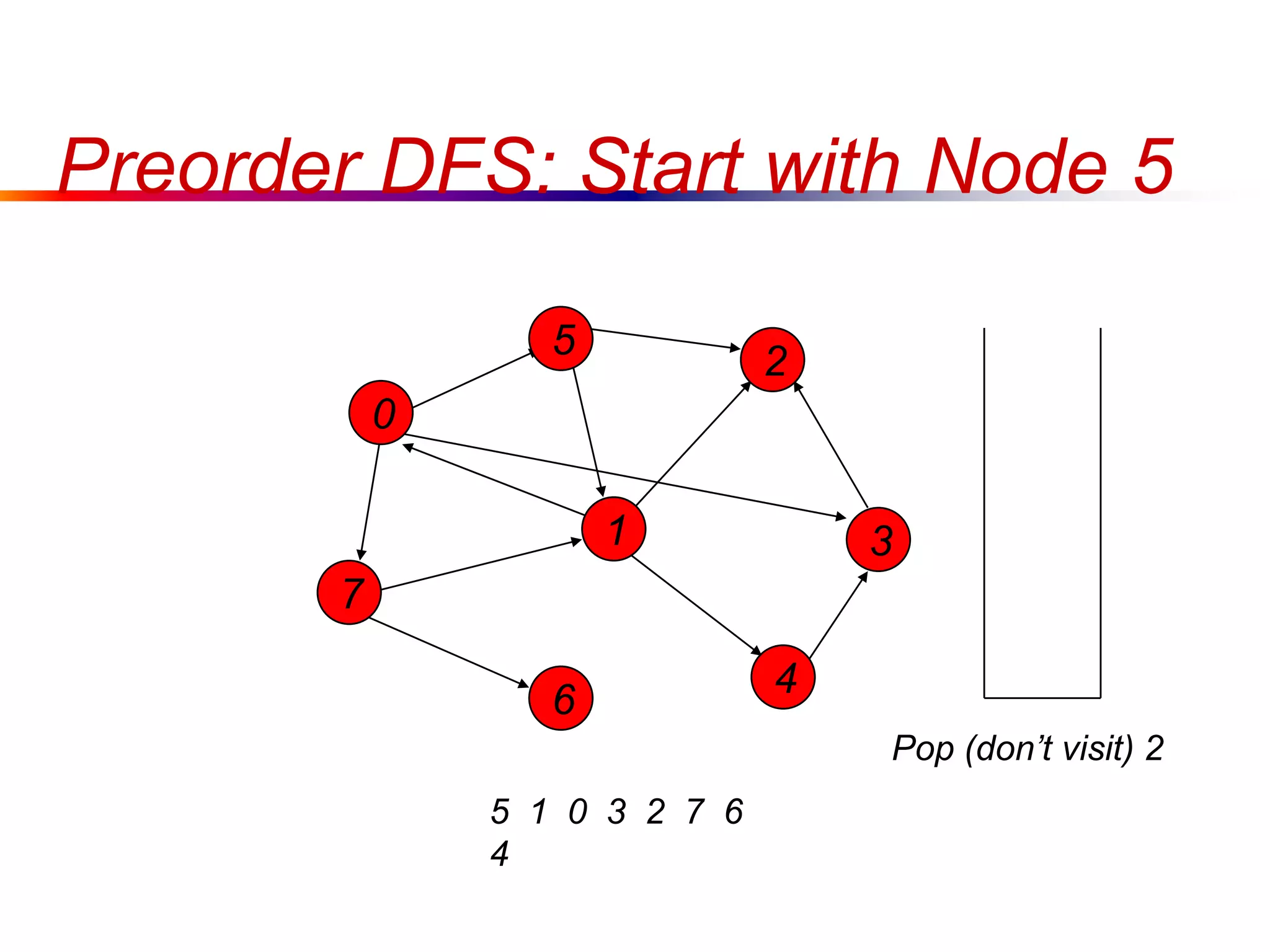
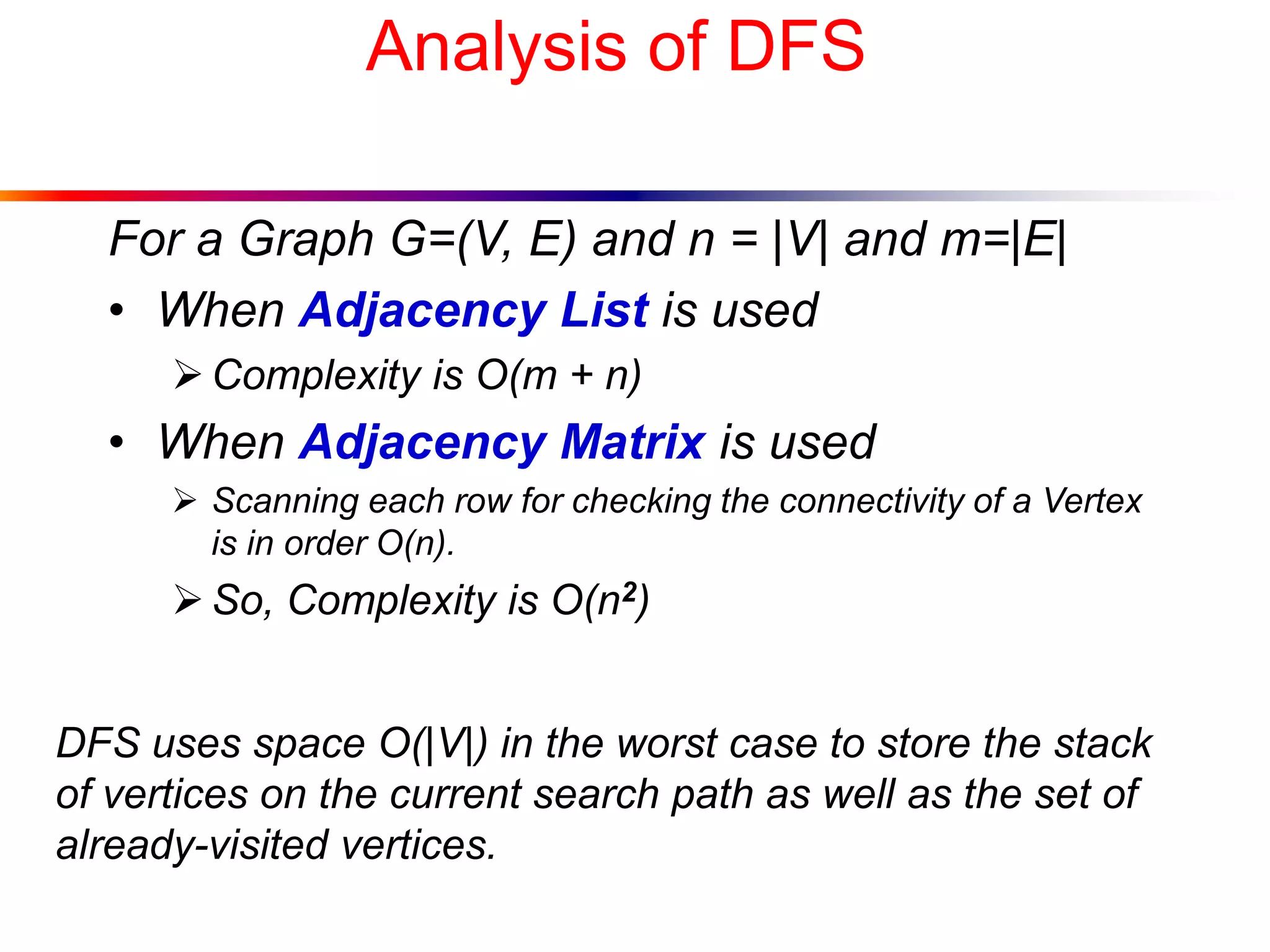

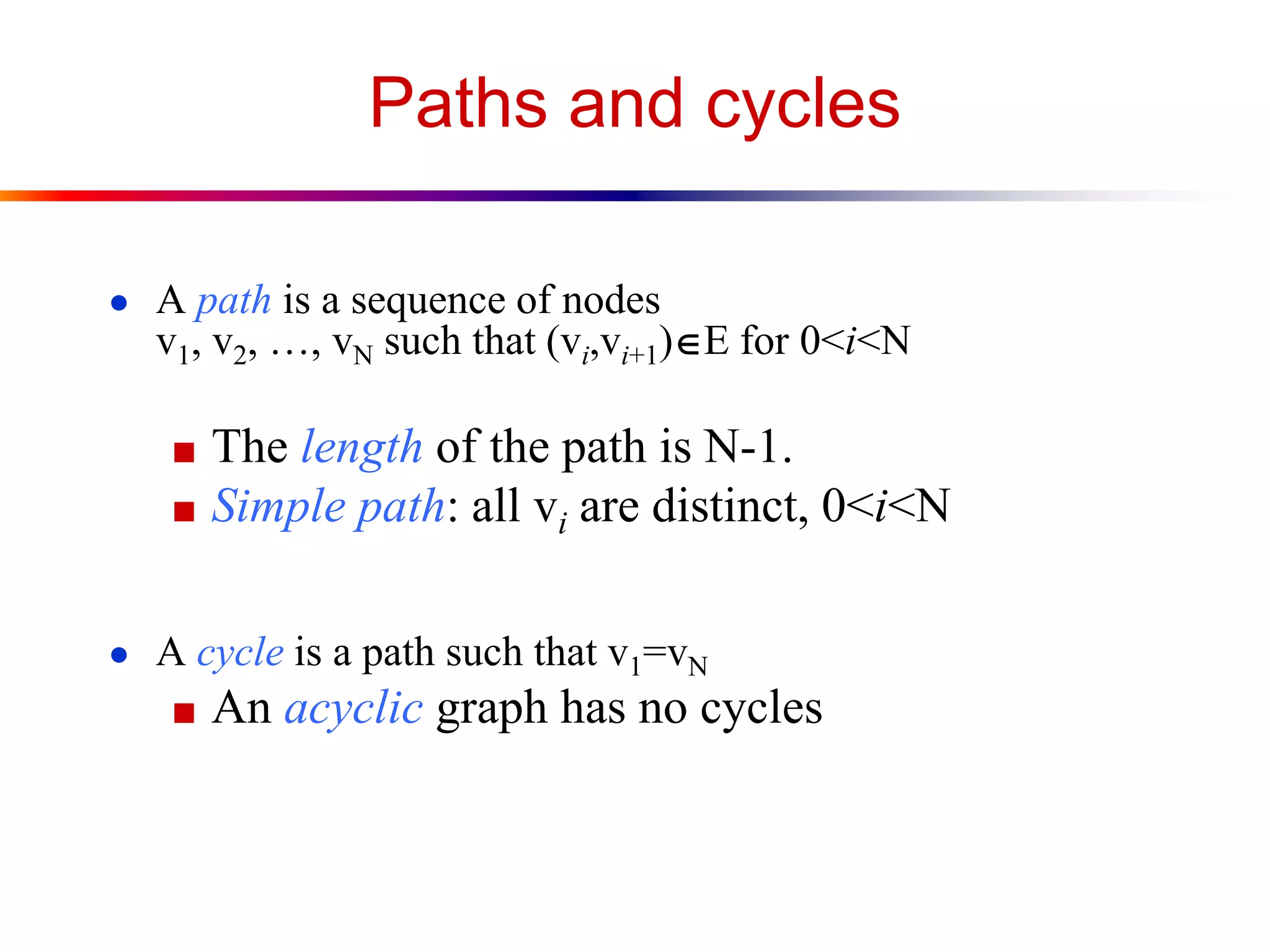
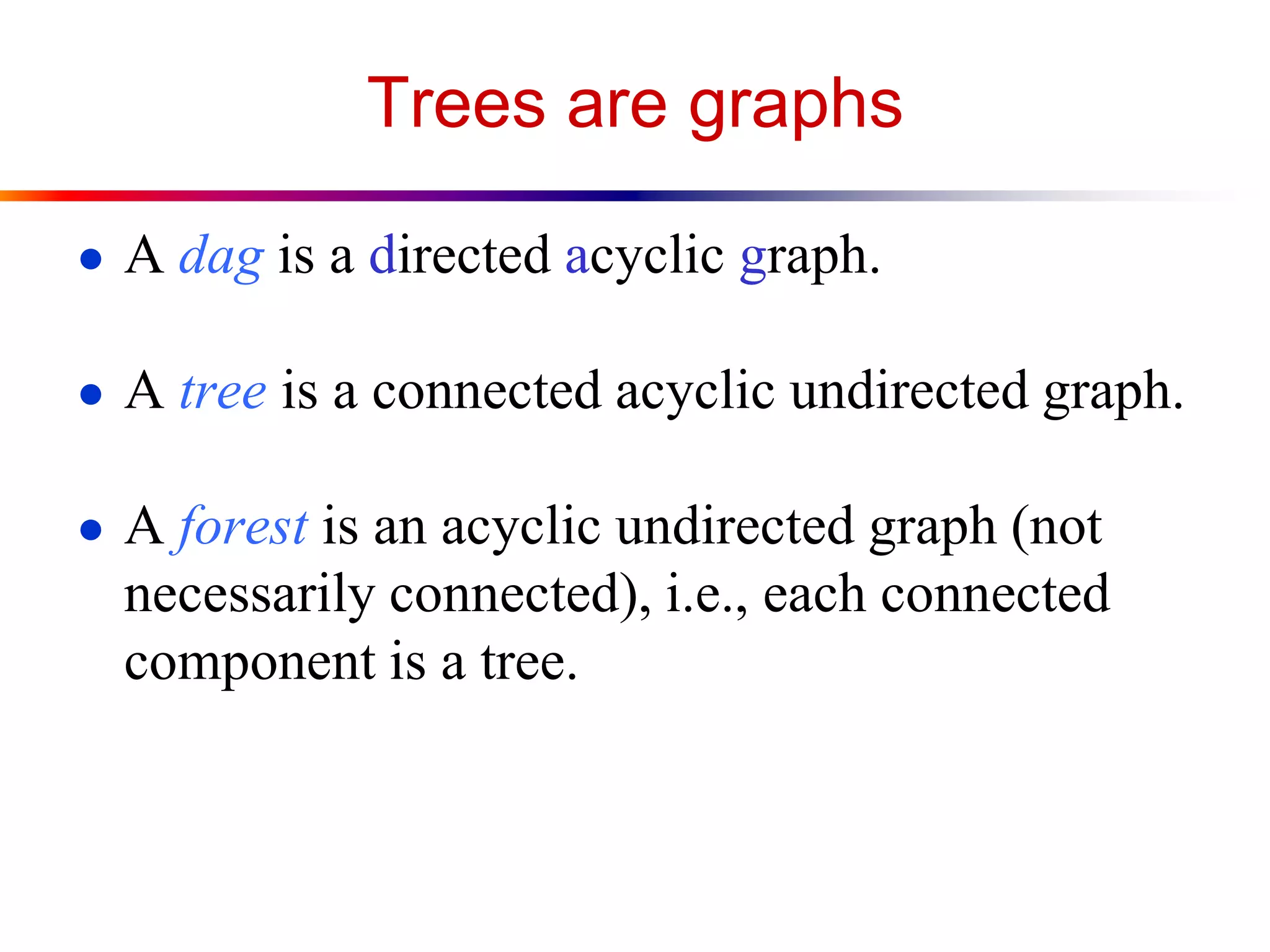
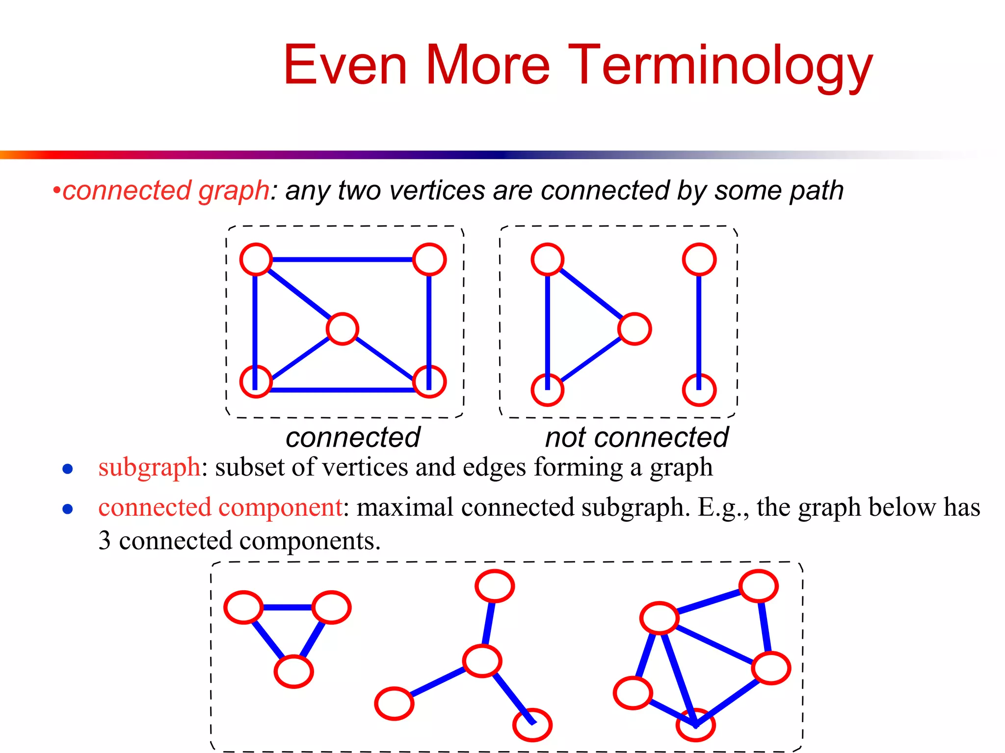
This document defines key graph concepts like paths, cycles, degrees of vertices, and different types of graphs like trees, forests, and directed acyclic graphs. It also describes common graph representations like adjacency matrices and lists. Finally, it covers graph traversal algorithms like breadth-first search and depth-first search, outlining their time complexities and providing examples of their process.


![Data Structures - Lecture 10 [Graphs]](https://cdn.slidesharecdn.com/ss_thumbnails/datastructures-lecture10graphs-150305004608-conversion-gate01-thumbnail.jpg?width=640&height=640&fit=bounds)