


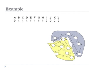
![Alternatives for Disjoint Sets
Can be implemented using lists, arrays, forest of trees
and forest of trees + heuristics
Simplest solutions: use arrays
set[1..n] = array with the representative of each element
in all the disjoint sets](https://image.slidesharecdn.com/adc9-101209123728-phpapp01/85/Algorithm-Design-and-Complexity-Course-9-35-320.jpg)
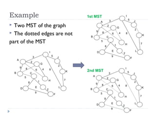
![Arrays as Disjoint Sets
Complexity?
MAKE-SET(u): Θ(1)
FIND-SET(u): Θ(1)
UNION(u, v): Θ(n)
Have to walk through all the elements of the smallest disjoint set and
change their representative to the one of the highest disjoint set!
Kruskal complexity?
Just return set[u]
Θ(m*logm + m + n2) = Θ(m*logm + n2)
Want better!](https://image.slidesharecdn.com/adc9-101209123728-phpapp01/85/Algorithm-Design-and-Complexity-Course-9-37-320.jpg)


![Prim - Pseudocode
Prim(G, w, s)
FOREACH (v∈V)
p[v] = NULL; d[v] = INF;
d[s] = 0
A=∅
S=∅
Q = PRIORITY-QUEUE(V, d)
// used only to denote the cut
// build a priority queue indexed by the vertices V
// with priorities in d[u] for each vertex
WHILE (!Q.EMPTY())
u = Q.EXTRACT-MIN()
// pick the light edge = safe edge
S = S U {u}
// add the current vertex to the other side of the cut
A = A U {(u, p[u])}
// add the current edge to the partial MST
FOREACH (v∈Adj[u])
IF (d[v] > w(u,v))
// found a better edge from S to v
d[v] = w(u,v)
// need to heapify-up the element!
// Q.DECREASE-KEY(v, w(u,v))
p[v] = u
RETURN A {(s, p(s))}](https://image.slidesharecdn.com/adc9-101209123728-phpapp01/85/Algorithm-Design-and-Complexity-Course-9-44-320.jpg)
![Prim – Remarks
Uses a priority queue in order to allow finding the light
edge for the cut (S, V S) as efficiently as possible
The vertices that are in the priority queue are the ones
in V S
d[v] contains the minimum weight of an edge that
connects v with any vertex from S (true for each vertex
that is still in the priority queue)
(p[u], u) is exactly this minimum weight edge!](https://image.slidesharecdn.com/adc9-101209123728-phpapp01/85/Algorithm-Design-and-Complexity-Course-9-45-320.jpg)


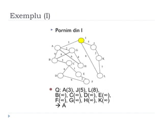
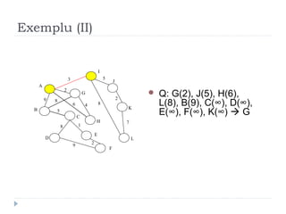
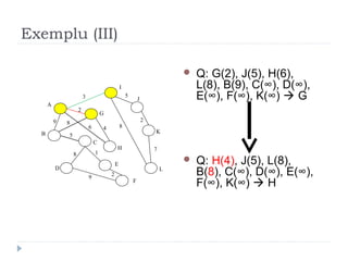
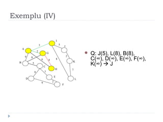
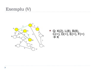
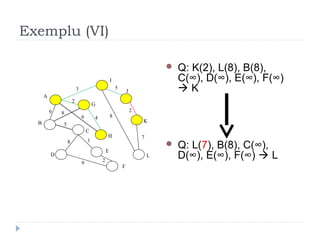
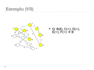
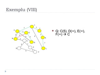
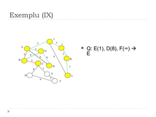


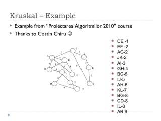
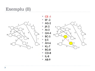
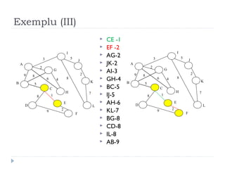
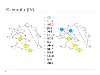
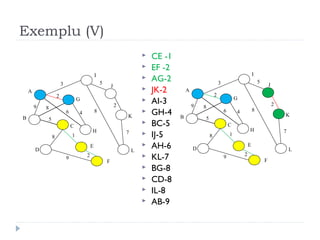
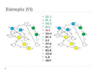
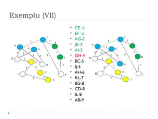
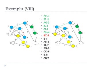
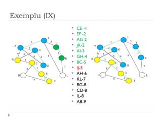
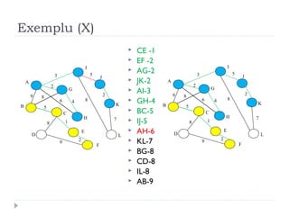
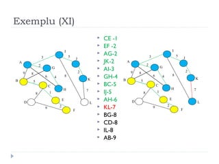
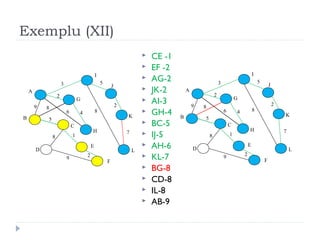
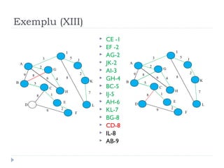
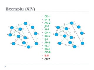
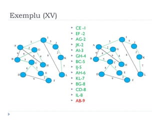
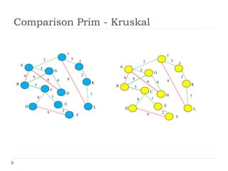
The document describes Kruskal's algorithm for finding the minimum spanning tree (MST) of a connected, undirected graph. Kruskal's algorithm works by sorting the edges by weight and then greedily adding edges to the MST one by one, skipping any edges that would create cycles. It uses the property that a minimum edge between disjoint components of the partial MST must be part of the overall MST. The runtime is O(ElogE) where E is the number of edges. An example run on a graph is shown step-by-step to demonstrate the algorithm.


![DAA-seminar-1[1].pptx Design and Analysis Of The Algorithm](https://cdn.slidesharecdn.com/ss_thumbnails/daa-seminar-11-250921155526-8ea0ea04-thumbnail.jpg?width=640&height=640&fit=bounds)