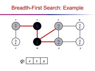
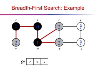
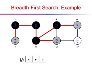
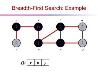
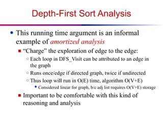
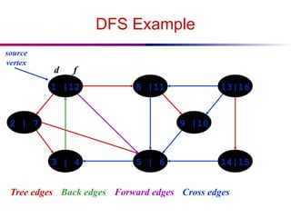
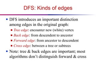
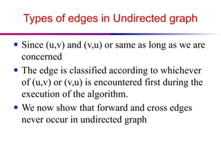
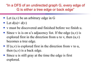
The document discusses the design and analysis of graph algorithms, focusing on breadth-first search (BFS) and depth-first search (DFS). It describes the representation of graphs, the methods of exploring vertices and edges, and analyzes the time complexities of both search algorithms. It also covers the distinctions between different types of edges in DFS and their implications for cycle detection in undirected graphs.

1. Design and Analysis of Algorithms
Graph Algorithms
Breadth first search and Depth first search

2. Graphs
● A graph G = (V, E)
■ V = set of vertices, E = set of edges
■ Dense graph: |E|  |V|2
; Sparse graph: |E|  |V|
■ Undirected graph:
○ Edge (u,v) = edge (v,u)
○ No self-loops
■ Directed graph:
○ Edge (u,v) goes from vertex u to vertex v, notated uv
■ A weighted graph associates weights with either
the edges or the vertices

3. Review: Representing Graphs
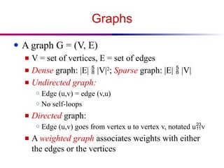
● Assume V = {1, 2, …, n}
● An adjacency matrix represents the graph as a
n x n matrix A:
■ A[i, j] = 1 if edge (i, j)  E (or weight of
edge)
= 0 if edge (i, j)  E
■ Storage requirements: O(V2
)
○ A dense representation
■ But, can be very efficient for small graphs
○ Especially if store just one bit/edge
○ Undirected graph: only need one diagonal of matrix

4. Review: Graph Searching
● Given: a graph G = (V, E), directed or
undirected
● Goal: methodically explore every vertex and
every edge
● Ultimately: build a tree on the graph
■ Pick a vertex as the root
■ Choose certain edges to produce a tree
■ Note: might also build a forest if graph is not
connected

5. Review: Breadth-First Search
● “Explore” a graph, turning it into a tree
■ One vertex at a time
■ Expand frontier of explored vertices across the
breadth of the frontier
● Builds a tree over the graph
■ Pick a source vertex to be the root
■ Find (“discover”) its children, then their children,
etc.

6. Review: Breadth-First Search
● will associate vertex “colors” to guide the
algorithm
■ White vertices have not been discovered
○ All vertices start out white
■ Grey vertices are discovered but not fully explored
○ They may be adjacent to white vertices
■ Black vertices are discovered and fully explored
○ They are adjacent only to black and gray vertices
● Explore vertices by scanning adjacency list of
grey vertices

7. Review: Breadth-First Search
BFS(G, s) {
initialize vertices;
Q = {s}; // Q is a queue; initialize to s
while (Q not empty) {
u = RemoveTop(Q);
for each v  u->adj {
if (v->color == WHITE)
v->color = GREY;
v->d = u->d + 1;
v->p = u;
Enqueue(Q, v);
}
u->color = BLACK;
}
}
What does v->p represent?
What does v->d represent?

8. Breadth-First Search: Example








r s t u
v w x y

9. Breadth-First Search: Example


0





r s t u
v w x y
s
Q:

10. Breadth-First Search: Example
1

0
1




r s t u
v w x y
w
Q: r

11. Breadth-First Search: Example
1

0
1
2
2


r s t u
v w x y
r
Q: t x

12. Breadth-First Search: Example
1
2
0
1
2
2


r s t u
v w x y
Q: t x v

13. Breadth-First Search: Example
1
2
0
1
2
2
3

r s t u
v w x y
Q: x v u

14. Breadth-First Search: Example
1
2
0
1
2
2
3
3
r s t u
v w x y
Q: v u y

15. Breadth-First Search: Example
1
2
0
1
2
2
3
3
r s t u
v w x y
Q: u y

16. Breadth-First Search: Example
1
2
0
1
2
2
3
3
r s t u
v w x y
Q: y

17. Breadth-First Search: Example
1
2
0
1
2
2
3
3
r s t u
v w x y
Q: Ø

18. BFS: The Code Again
BFS(G, s) {
initialize vertices;
Q = {s};
while (Q not empty) {
u = RemoveTop(Q);
for each v  u->adj {
if (v->color == WHITE)
v->color = GREY;
v->d = u->d + 1;
v->p = u;
Enqueue(Q, v);
}
u->color = BLACK;
}
}
What will be the running time?
Touch every vertex: O(V)
u = every vertex, but only once
(Why?)
So v = every vertex
that appears in
some other vert’s
adjacency list
Total running time: O(V+E)

19. BFS: The Code Again
BFS(G, s) {
initialize vertices;
Q = {s};
while (Q not empty) {
u = RemoveTop(Q);
for each v  u->adj {
if (v->color == WHITE)
v->color = GREY;
v->d = u->d + 1;
v->p = u;
Enqueue(Q, v);
}
u->color = BLACK;
}
}

20. Breadth-First Search: Properties
● BFS calculates the shortest-path distance to
the source node
■ Shortest-path distance (s,v) = minimum number
of edges from s to v, or  if v not reachable from s
■ Proof given in the book (p. 472-5)
● BFS builds breadth-first tree, in which paths to
root represent shortest paths in G
■ Thus can use BFS to calculate shortest path from
one vertex to another in O(V+E) time

21. Depth-First Search
● Depth-first search is another strategy for
exploring a graph
■ Explore “deeper” in the graph whenever possible
■ Edges are explored out of the most recently
discovered vertex v that still has unexplored edges
■ When all of v’s edges have been explored,
backtrack to the vertex from which v was
discovered

22. Depth-First Search
● Vertices initially colored white
● Then colored gray when discovered
● Then black when finished

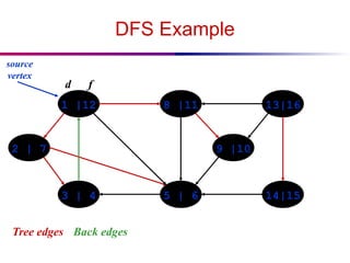
23. Depth-First Search: The Code
DFS(G)
{
for each vertex u  G->V
{
u->color = WHITE;
}
time = 0;
for each vertex u  G->V
{
if (u->color == WHITE)
DFS_Visit(u);
}
}
DFS_Visit(u)
{
u->color = GREY;
time = time+1;
u->d = time;
for each v  u->Adj[]
{
if (v->color == WHITE)
DFS_Visit(v);
}
u->color = BLACK;
time = time+1;
u->f = time;
}

24. Depth-First Search: The Code
DFS(G)
{
for each vertex u  G->V
{
u->color = WHITE;
}
time = 0;
for each vertex u  G->V
{
if (u->color == WHITE)
DFS_Visit(u);
}
}
DFS_Visit(u)
{
u->color = GREY;
time = time+1;
u->d = time;
for each v  u->Adj[]
{
if (v->color == WHITE)
DFS_Visit(v);
}
u->color = BLACK;
time = time+1;
u->f = time;
}
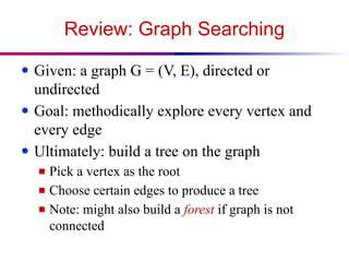
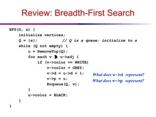
What does u->d represent?

25. Depth-First Search: The Code
DFS(G)
{
for each vertex u  G->V
{
u->color = WHITE;
}
time = 0;
for each vertex u  G->V
{
if (u->color == WHITE)
DFS_Visit(u);
}
}
DFS_Visit(u)
{
u->color = GREY;
time = time+1;
u->d = time;
for each v  u->Adj[]
{
if (v->color == WHITE)
DFS_Visit(v);
}
u->color = BLACK;
time = time+1;
u->f = time;
}
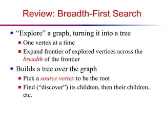
What does u->f represent?

26. Depth-First Search: The Code
DFS(G)
{
for each vertex u  G->V
{
u->color = WHITE;
}
time = 0;
for each vertex u  G->V
{
if (u->color == WHITE)
DFS_Visit(u);
}
}
DFS_Visit(u)
{
u->color = GREY;
time = time+1;
u->d = time;
for each v  u->Adj[]
{
if (v->color == WHITE)
DFS_Visit(v);
}
u->color = BLACK;
time = time+1;
u->f = time;
}
Will all vertices eventually be colored black?

27. Depth-First Search: The Code
DFS(G)
{
for each vertex u  G->V
{
u->color = WHITE;
}
time = 0;
for each vertex u  G->V
{
if (u->color == WHITE)
DFS_Visit(u);
}
}
DFS_Visit(u)
{
u->color = GREY;
time = time+1;
u->d = time;
for each v  u->Adj[]
{
if (v->color == WHITE)
DFS_Visit(v);
}
u->color = BLACK;
time = time+1;
u->f = time;
}
What will be the running time?

28. Depth-First Search: The Code
DFS(G)
{
for each vertex u  G->V
{
u->color = WHITE;
}
time = 0;
for each vertex u  G->V
{
if (u->color == WHITE)
DFS_Visit(u);
}
}
DFS_Visit(u)
{
u->color = GREY;
time = time+1;
u->d = time;
for each v  u->Adj[]
{
if (v->color == WHITE)
DFS_Visit(v);
}
u->color = BLACK;
time = time+1;
u->f = time;
}
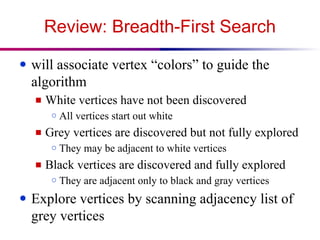
Running time: O(n2
) because call DFS_Visit on each vertex,
and the loop over Adj[] can run as many as |V| times

29. Depth-First Search: The Code
DFS(G)
{
for each vertex u  G->V
{
u->color = WHITE;
}
time = 0;
for each vertex u  G->V
{
if (u->color == WHITE)
DFS_Visit(u);
}
}
DFS_Visit(u)
{
u->color = GREY;
time = time+1;
u->d = time;
for each v  u->Adj[]
{
if (v->color == WHITE)
DFS_Visit(v);
}
u->color = BLACK;
time = time+1;
u->f = time;
}
BUT, there is actually a tighter bound.
How many times will DFS_Visit() actually be called?

30. Depth-First Search: The Code
DFS(G)
{
for each vertex u  G->V
{
u->color = WHITE;
}
time = 0;
for each vertex u  G->V
{
if (u->color == WHITE)
DFS_Visit(u);
}
}
DFS_Visit(u)
{
u->color = GREY;
time = time+1;
u->d = time;
for each v  u->Adj[]
{
if (v->color == WHITE)
DFS_Visit(v);
}
u->color = BLACK;
time = time+1;
u->f = time;
}
So, running time of DFS = O(V+E)

31. Depth-First Sort Analysis
● This running time argument is an informal
example of amortized analysis
■ “Charge” the exploration of edge to the edge:
○ Each loop in DFS_Visit can be attributed to an edge in
the graph
○ Runs once/edge if directed graph, twice if undirected
○ Thus loop will run in O(E) time, algorithm O(V+E)
 Considered linear for graph, b/c adj list requires O(V+E) storage
■ Important to be comfortable with this kind of
reasoning and analysis

32. DFS Example
source
vertex

33. DFS Example
1 | | |
|
|
|
| |
source
vertex
d f

34. DFS Example
1 | | |
|
|
|
2 | |
source
vertex
d f

35. DFS Example
1 | | |
|
|
3 |
2 | |
source
vertex
d f

36. DFS Example
1 | | |
|
|
3 | 4
2 | |
source
vertex
d f

37. DFS Example
1 | | |
|
5 |
3 | 4
2 | |
source
vertex
d f

38. DFS Example
1 | | |
|
5 | 6
3 | 4
2 | |
source
vertex
d f

39. DFS Example
1 | 8 | |
|
5 | 6
3 | 4
2 | 7 |
source
vertex
d f

40. DFS Example
1 | 8 | |
|
5 | 6
3 | 4
2 | 7 |
source
vertex
d f

41. DFS Example
1 | 8 | |
|
5 | 6
3 | 4
2 | 7 9 |
source
vertex
d f
What is the structure of the grey vertices?
What do they represent?

42. DFS Example
1 | 8 | |
|
5 | 6
3 | 4
2 | 7 9 |10
source
vertex
d f

43. DFS Example
1 | 8 |11 |
|
5 | 6
3 | 4
2 | 7 9 |10
source
vertex
d f

44. DFS Example
1 |12 8 |11 |
|
5 | 6
3 | 4
2 | 7 9 |10
source
vertex
d f

45. DFS Example
1 |12 8 |11 13|
|
5 | 6
3 | 4
2 | 7 9 |10
source
vertex
d f

46. DFS Example
1 |12 8 |11 13|
14|
5 | 6
3 | 4
2 | 7 9 |10
source
vertex
d f

47. DFS Example
1 |12 8 |11 13|
14|15
5 | 6
3 | 4
2 | 7 9 |10
source
vertex
d f

48. DFS Example
1 |12 8 |11 13|16
14|15
5 | 6
3 | 4
2 | 7 9 |10
source
vertex
d f

49. DFS: Kinds of edges
● DFS introduces an important distinction
among edges in the original graph:
■ Tree edge: encounter new (white) vertex
○ The tree edges form a spanning forest
○ Can tree edges form cycles? Why or why not?

50. DFS Example
1 |12 8 |11 13|16
14|15
5 | 6
3 | 4
2 | 7 9 |10
source
vertex
d f
Tree edges

51. DFS: Kinds of edges
● DFS introduces an important distinction
among edges in the original graph:
■ Tree edge: encounter new (white) vertex
■ Back edge: from descendent to ancestor
○ Encounter a grey vertex (grey to grey)

52. DFS Example
1 |12 8 |11 13|16
14|15
5 | 6
3 | 4
2 | 7 9 |10
source
vertex
d f
Tree edges Back edges

53. DFS: Kinds of edges
● DFS introduces an important distinction
among edges in the original graph:
■ Tree edge: encounter new (white) vertex
■ Back edge: from descendent to ancestor
■ Forward edge: from ancestor to descendent
○ Not a tree edge, though
○ From grey node to black node

54. DFS Example
1 |12 8 |11 13|16
14|15
5 | 6
3 | 4
2 | 7 9 |10
source
vertex
d f
Tree edges Back edges Forward edges

55. DFS: Kinds of edges
● DFS introduces an important distinction
among edges in the original graph:
■ Tree edge: encounter new (white) vertex
■ Back edge: from descendent to ancestor
■ Forward edge: from ancestor to descendent
■ Cross edge: between a tree or subtrees
○ From a grey node to a black node

56. DFS Example
1 |12 8 |11 13|16
14|15
5 | 6
3 | 4
2 | 7 9 |10
source
vertex
d f
Tree edges Back edges Forward edges Cross edges

57. DFS: Kinds of edges
● DFS introduces an important distinction
among edges in the original graph:
■ Tree edge: encounter new (white) vertex
■ Back edge: from descendent to ancestor
■ Forward edge: from ancestor to descendent
■ Cross edge: between a tree or subtrees
● Note: tree & back edges are important; most
algorithms don’t distinguish forward & cross

58. Types of edges in Undirected graph
● Since (u,v) and (v,u) or same as long as we are
concerned
● The edge is classified according to whichever
of (u,v) or (v,u) is encountered first during the
execution of the algorithm.
● We now show that forward and cross edges
never occur in undirected graph

59. “In a DFS of an undirected graph G, every edge of
G is either a tree edge or back edge”
● Let (u,v) be an arbitrary edge in G
● Let d(u)< d(v)
● v must be discovered and finished before we finish u.
● Since v is is on u’s adjacency list. If the edge (u,v) is
explored first in the direction from u to v, then (u,v)
becomes a tree edge.
● If (u,v) is explored first in the direction from v to u,
then (u,v) is a back edge.
● Since u is still gray at the time the edge is first
explored.

60. DFS And Graph Cycles
● Thm: An undirected graph is acyclic iff a DFS
yields no back edges
■ If acyclic, no back edges (because a back edge
implies a cycle
■ If no back edges, acyclic
○ No back edges implies only tree edges (Why?)
○ Only tree edges implies we have a tree or a forest
○ Which by definition is acyclic
● Thus, can run DFS to find whether a graph has
a cycle

61. DFS And Cycles
● How would you modify the code to detect cycles?
DFS(G)
{
for each vertex u  G->V
{
u->color = WHITE;
}
time = 0;
for each vertex u  G->V
{
if (u->color == WHITE)
DFS_Visit(u);
}
}
DFS_Visit(u)
{
u->color = GREY;
time = time+1;
u->d = time;
for each v  u->Adj[]
{
if (v->color == WHITE)
DFS_Visit(v);
}
u->color = BLACK;
time = time+1;
u->f = time;
}

62. DFS And Cycles
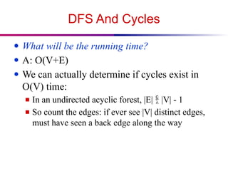
● What will be the running time?
DFS(G)
{
for each vertex u  G->V
{
u->color = WHITE;
}
time = 0;
for each vertex u  G->V
{
if (u->color == WHITE)
DFS_Visit(u);
}
}
DFS_Visit(u)
{
u->color = GREY;
time = time+1;
u->d = time;
for each v  u->Adj[]
{
if (v->color == WHITE)
DFS_Visit(v);
}
u->color = BLACK;
time = time+1;
u->f = time;
}

63. DFS And Cycles
● What will be the running time?
● A: O(V+E)
● We can actually determine if cycles exist in
O(V) time:
■ In an undirected acyclic forest, |E|  |V| - 1
■ So count the edges: if ever see |V| distinct edges,
must have seen a back edge along the way

64. Directed Acyclic Graphs
● A directed acyclic graph or DAG is a directed
graph with no directed cycles:

65. DFS and DAGs
● A directed graph G is acyclic iff a DFS of G
yields no back edges.
● A back edge implies existence of a cycle.

66. Topological Sort
● Topological sort of a DAG:
■ Linear ordering of all vertices in graph G such that
vertex u comes before vertex v if edge (u, v)  G
● Real-world example: getting dressed

67. Getting Dressed
Socks
Shoes
Pants
Belt
Shirt
Watch
Tie
Jacket

68. Getting Dressed
Socks
Shoes
Pants
Belt
Shirt
Watch
Tie
Jacket
Socks Pants Shoes Watch Shirt Belt Tie Jacket

69. Topological Sort Algorithm
Topological-Sort()
{
Run DFS
When a vertex is finished, output it
Vertices are output in reverse
topological order
}
● Time: O(V+E)
● Correctness: Want to prove that
(u,v)  G  uf > vf

70. Correctness of Topological Sort
● Claim: (u,v)  G  uf > vf
■ When (u,v) is explored, u is grey
○ v = grey  (u,v) is back edge. Contradiction (Why?)
○ v = white  v becomes descendent of u  vf < uf
(since must finish v before backtracking and finishing
u)
○ v = black  v already finished  vf < uf